About ModelingToolKit.jl/GG backend

ModelingToolkit.jl of GG backend requires usingSymbolics.jl of GG backend:

] add https://github.com/thautwarm/Symbolics.jl

Pros and Cons Using GG v0.3+ for MTK

Pros:

GG v0.3 can compute the small common parts of values and cache them once, which significantly reduces startup latency and memory usage.

For instance, multiple Julia expressions derived from begin x = 1; y = begin x + 1 end end but contains different line number nodes can share nearly the same cache. Only LineNumberNodes are stored and cached multiple times.

Cons:

In order to share the same caches for more values from different packages, GG holds only one cache store which is inside GG itself. As a consequence, generated functions from GG cannot get pre-compiled at the caller packages.

The cache store is runtime-specific, which means that GG functions do not work properly with serialization.

ModelingToolkit.jl

ModelingToolkit.jl is a modeling framework for high-performance symbolic-numeric computation in scientific computing and scientific machine learning. It allows for users to give a high-level description of a model for symbolic preprocessing to analyze and enhance the model. ModelingToolkit can automatically generate fast functions for model components like Jacobians and Hessians, along with automatically sparsifying and parallelizing the computations. Automatic transformations, such as index reduction, can be applied to the model to make it easier for numerical solvers to handle.

For information on using the package, see the stable documentation. Use the in-development documentation for the version of the documentation which contains the unreleased features.

High-Level Examples

First, let's define a second order riff on the Lorenz equations, symbolically lower it to a first order system, symbolically generate the Jacobian function for the numerical integrator, and solve it.

using ModelingToolkit, OrdinaryDiffEq

@parameters t σ ρ β
@variables x(t) y(t) z(t)
D = Differential(t)

eqs = [D(D(x)) ~ σ*(y-x),
       D(y) ~ x*(ρ-z)-y,
       D(z) ~ x*y - β*z]

sys = ODESystem(eqs)
sys = ode_order_lowering(sys)

u0 = [D(x) => 2.0,
      x => 1.0,
      y => 0.0,
      z => 0.0]

p  = [σ => 28.0,
      ρ => 10.0,
      β => 8/3]

tspan = (0.0,100.0)
prob = ODEProblem(sys,u0,tspan,p,jac=true)
sol = solve(prob,Tsit5())
using Plots; plot(sol,vars=(x,y))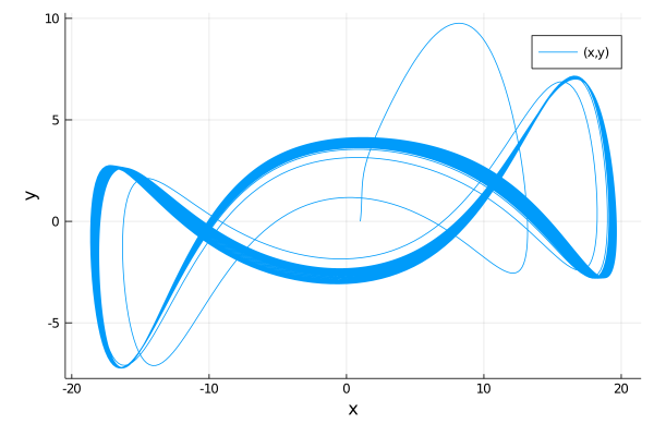

This automatically will have generated fast Jacobian functions, making it more optimized than directly building a function. In addition, we can then use ModelingToolkit to compose multiple ODE subsystems. Now, let's define two interacting Lorenz equations and simulate the resulting Differential-Algebraic Equation (DAE):

using ModelingToolkit, OrdinaryDiffEq

@parameters t σ ρ β
@variables x(t) y(t) z(t)
D = Differential(t)

eqs = [D(x) ~ σ*(y-x),
       D(y) ~ x*(ρ-z)-y,
       D(z) ~ x*y - β*z]

lorenz1 = ODESystem(eqs,name=:lorenz1)
lorenz2 = ODESystem(eqs,name=:lorenz2)

@variables a
@parameters γ
connections = [0 ~ lorenz1.x + lorenz2.y + a*γ]
connected = ODESystem(connections,t,[a],[γ],systems=[lorenz1,lorenz2])

u0 = [lorenz1.x => 1.0,
      lorenz1.y => 0.0,
      lorenz1.z => 0.0,
      lorenz2.x => 0.0,
      lorenz2.y => 1.0,
      lorenz2.z => 0.0,
      a => 2.0]

p  = [lorenz1.σ => 10.0,
      lorenz1.ρ => 28.0,
      lorenz1.β => 8/3,
      lorenz2.σ => 10.0,
      lorenz2.ρ => 28.0,
      lorenz2.β => 8/3,
      γ => 2.0]

tspan = (0.0,100.0)
prob = ODEProblem(connected,u0,tspan,p)
sol = solve(prob,Rodas4())

using Plots; plot(sol,vars=(a,lorenz1.x,lorenz2.z))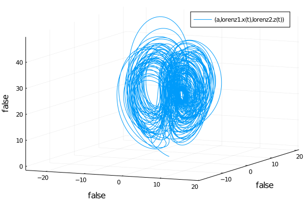

Citation

If you use ModelingToolkit.jl in your research, please cite this paper:

@misc{ma2021modelingtoolkit,
      title={ModelingToolkit: A Composable Graph Transformation System For Equation-Based Modeling},
      author={Yingbo Ma and Shashi Gowda and Ranjan Anantharaman and Chris Laughman and Viral Shah and Chris Rackauckas},
      year={2021},
      eprint={2103.05244},
      archivePrefix={arXiv},
      primaryClass={cs.MS}
}