JenksGTiff

Apply Jenks Natural Breaks on Geotiff files and get output image with graduated symbology.

Compute "natural breaks" (Jenks algorithm) on geotiff by preprocessing the image and thus reducing the runtime to calculate breaks while keeping the output almost more than 90% accurate to the natural break values of original dataset.

Intented compatibility: CPython 2.7+ and 3.4+

Required Dependancies:

GDAL :

pip install GDAL

Numpy :

pip install python-numpy

matplotlib :

pip install matplotlib
or    
sudo apt-get install python-matplotlib

jenkspy :

pip install jenkspy

Installation:

Download the zip file for the python package from github.

Unzip the folder to temporary location.

ubuntu@ubuntu:~$ cd tmp    
ubuntu@ubuntu:~/tmp$ unzip jenksGTiff.zip    
ubuntu@ubuntu:~/tmp$ cd jenksGTiff    
ubuntu@ubuntu:~/tmp/jenksGTiff$ pip install .

if you get an EnvironmentError: [Errno 13] Permission denied:, use

ubuntu@ubuntu:~/tmp/jenksGTiff$ pip install . --user

Usage :

>>> import jenksGTiff
>>> jenksGTiff.__all__
['clear_all', 'importGTiff', 'RemoveNoData', 'ReducedArray', 'JenksGTiff', 'DataStats', 'compareStats', 'histogram', 'exportGTiff']
>>> breaks, array, array_short = jenksGTiff.JenksGTiff('\pwd\input.tif', n_classes, NoDataVal=0, sample_size_ratio=0.1)
>>> breaks
[-0.9921568632125854, -0.37254902720451355, -0.05882352963089943, 0.13725490868091583, 0.26274511218070984, 0.40392157435417175]

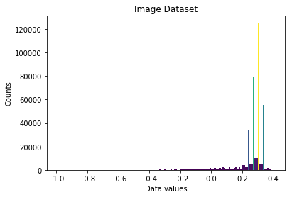
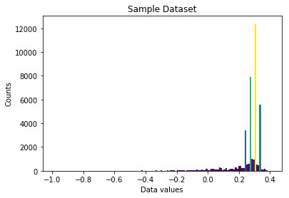
Since the image dataset was reduced to a small sample dataset, we compare both the stats and plot histograms.

>>> jenksGTiff.compareStats(array, array_short)
Stats Measures - Value (original dataset) - Value (Sample dataset) 

DataCount : 393868 : 39387
Minimum : -0.99215686 : -0.99215686
Maximum : 0.40392157 : 0.40392157
Sum : 102931.59580400819 : 10252.694481091574
Mean : 0.26133528 : 0.26030654
Median : 0.29411766 : 0.29411766
StandardDeviation : 0.11551328 : 0.117199086

>>> jenksGTiff.histogram(array, 'Image Dataset', bins=134)

>>> jenksGTiff.histogram(array_short, 'Sample Dataset', bins=134)

>>> new_value = jenksGTiff.exportGTiff('\pwd\input.tiff','\cwd\output.tif', breaks, NoDataVal=0)

This should give us the output geotiff file.

Benchmark against original or larger dataset:

In [1]: import timeit

In [2]: %timeit jenksGTiff.JenksGTiff('\pwd\input.tif', n_classes=5, NoDataVal=0, sample_size_ratio=0.1)
5.62 s ± 45.4 ms per loop (mean ± std. dev. of 7 runs, 1 loop each)

In [3]: %timeit jenksGTiff.JenksGTiff('\pwd\input.tif', n_classes=5, NoDataVal=0, sample_size_ratio=0.2)
25.7 s ± 1.51 s per loop (mean ± std. dev. of 7 runs, 1 loop each)

It is possible to obtain the Natural Breaks just with a sample dataset that is 10% of the original dataset. Running the algorithm on 10% sample dataset is ~4.6X faster than that compared to running on 20% sample dataset. This brings down the runtime to calculate the breaks significantly compared to running the whole dataset.

Author:

Nikhil S Hubballi