Example: Parallel optimization using scikit optimize

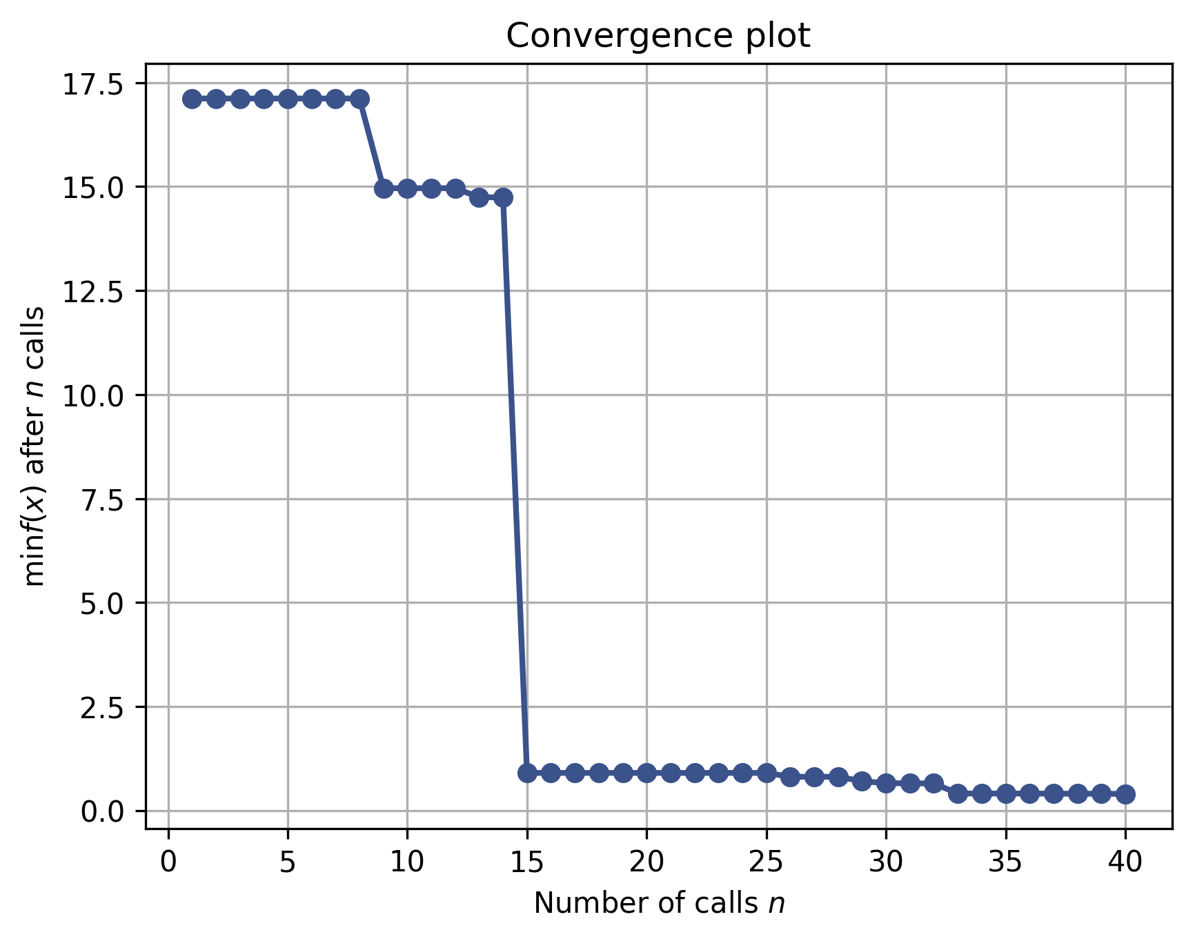
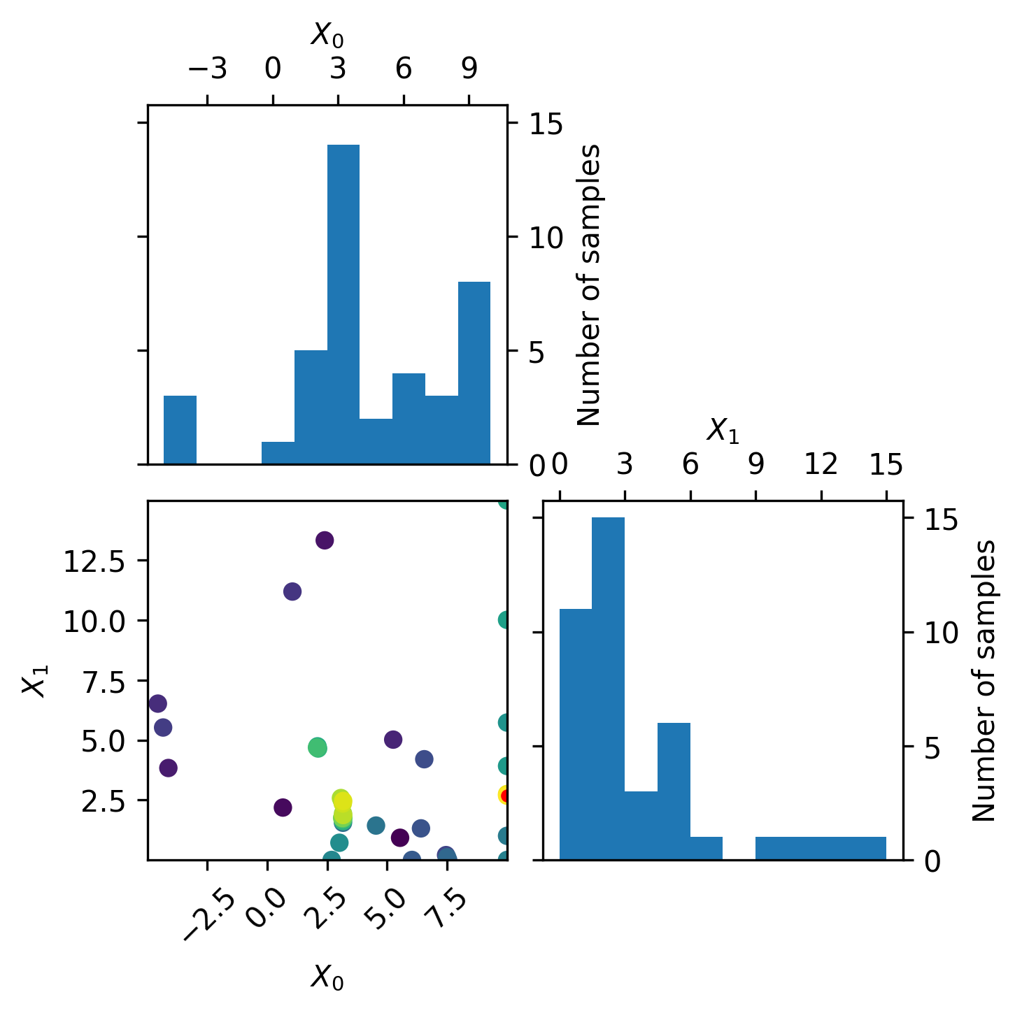
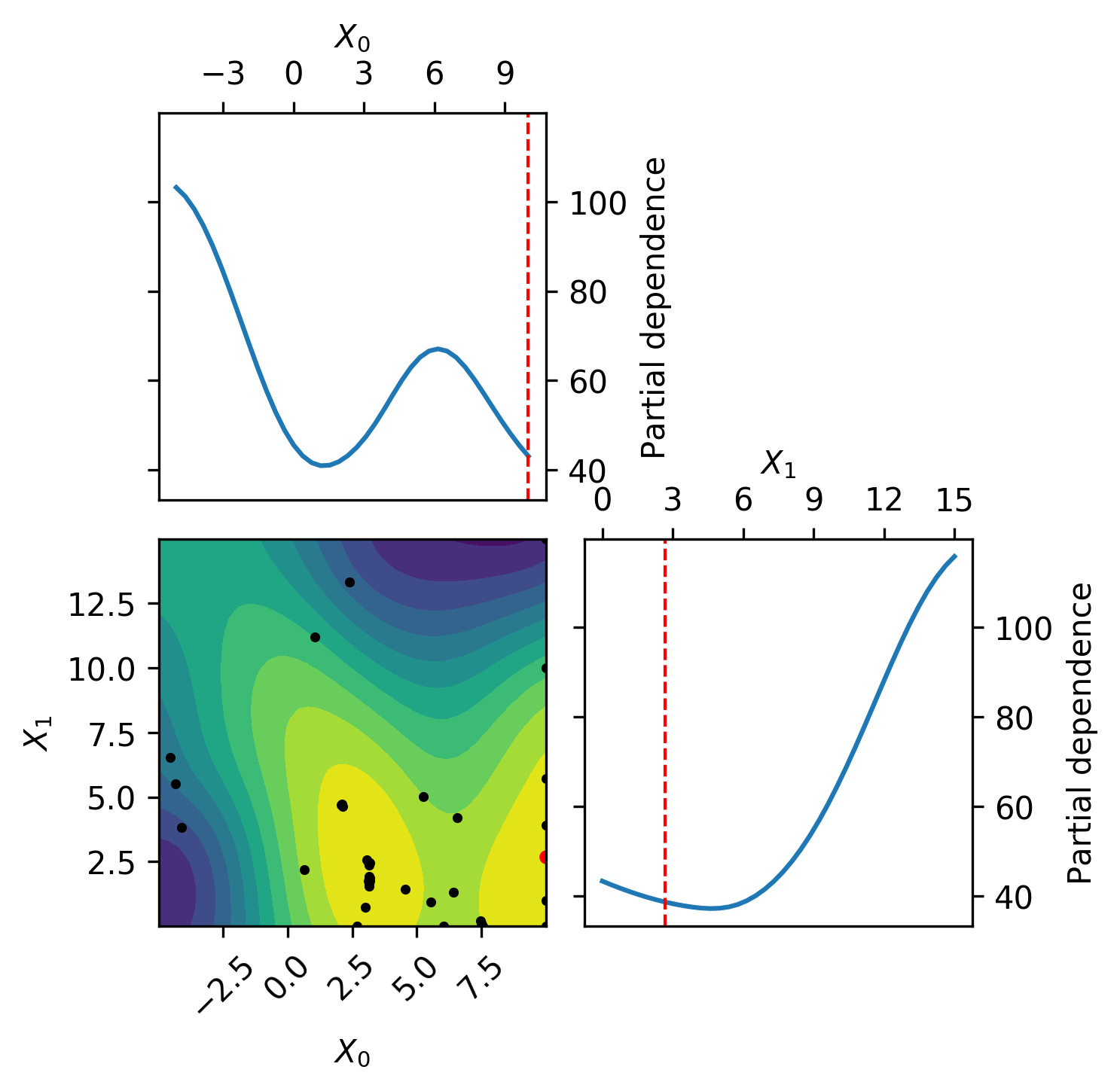
This toy example demonstrates parallel optimization using scikit optimize and law workflows.

In a real world example the objective will likely be a expensive to compute function like a neural network training or other computational demanding task. Here we will use the branin function as a benchmark.

For more information about the optimization strategy used in this example take a look at this scikit optimize tutorial.

Resources: luigi, law, scikit optimize, matplotlib

There are multiple ways to setup and run this example:

1. Docker: docker run -ti riga/law:example loremipsum
2. Local: source setup.sh

1. Install dependencies for this example

pip install luigi scikit-optimize matplotlib

2. Source the setup script (just sets up some variables)

source setup.sh

3. Let law index your the tasks and their parameters (for autocompletion)

law index --verbose

You should see:

loading tasks from 1 module(s)
loading module 'tasks', done

module 'tasks', 3 task(s):
    - Optimizer
    - OptimizerPlot
    - Objective

written 3 task(s) to index file '/examplepath/.law/index'

4. Check the status of the OptimizerPlot task

law run OptimizerPlot --print-status -1

No tasks ran so far, so no output target should exist yet. You will see this output:

print task status with max_depth -1 and target_depth 0

> check status of OptimizerPlot(branch=-1, iterations=10, n_parallel=4, n_initial_points=10, plot_objective=True)
|   - check TargetCollection(len=10, threshold=1.0)
|     -> absent (0/10)

The -1 value tells law to recursively check the task status. Given a positive number, law stops at that level. The task itself has a depth of 0.

5. Run the OptimizerPlot task

law run OptimizerPlot --iterations 10 --n-initial-points 10 --n-parallel 4

This should take a minute to process. You can see the plots being created after each optimization step at data/OptimizerPlot.

By default, this example uses a local scheduler, which - by definition - offers no visualization tools in the browser. If you want to see how the task tree is built and subsequently run, run luigid in a second terminal. This will start a central scheduler at localhost:8082 (the default address). To inform tasks (or rather workers) about the scheduler, either add --local-scheduler False to the law run command, or set the local-scheduler value in the [luigi_core] config section in the law.cfg file to False.

6. Check the status again

law run OptimizerPlot --print-status -1

When the optimization succeeded, all output targets should exist:

print task status with max_depth -1 and target_depth 0

> check status of OptimizerPlot(branch=-1, iterations=10, n_parallel=4, n_initial_points=10, plot_objective=True)
|   - check TargetCollection(len=10, threshold=1.0)
|     -> existent (10/10)

7. Look at the results

ls data/OptimizerPlot

Convergence of the optimization

Sampled points

Pairwise partial dependence plot of the objective function