cycloidgen

Parametric cycloidal drive design

A desktop app that takes a handful of parameters — or a set of requirements —
runs the drive live in 2D and 3D, checks it, sizes it, and writes DXF, SVG, STEP,
STL, a looping animation, a bill of materials and a PDF dossier.

Download  ·  pip install cycloidgen  ·  Python API  ·  The checks  ·  Changelog

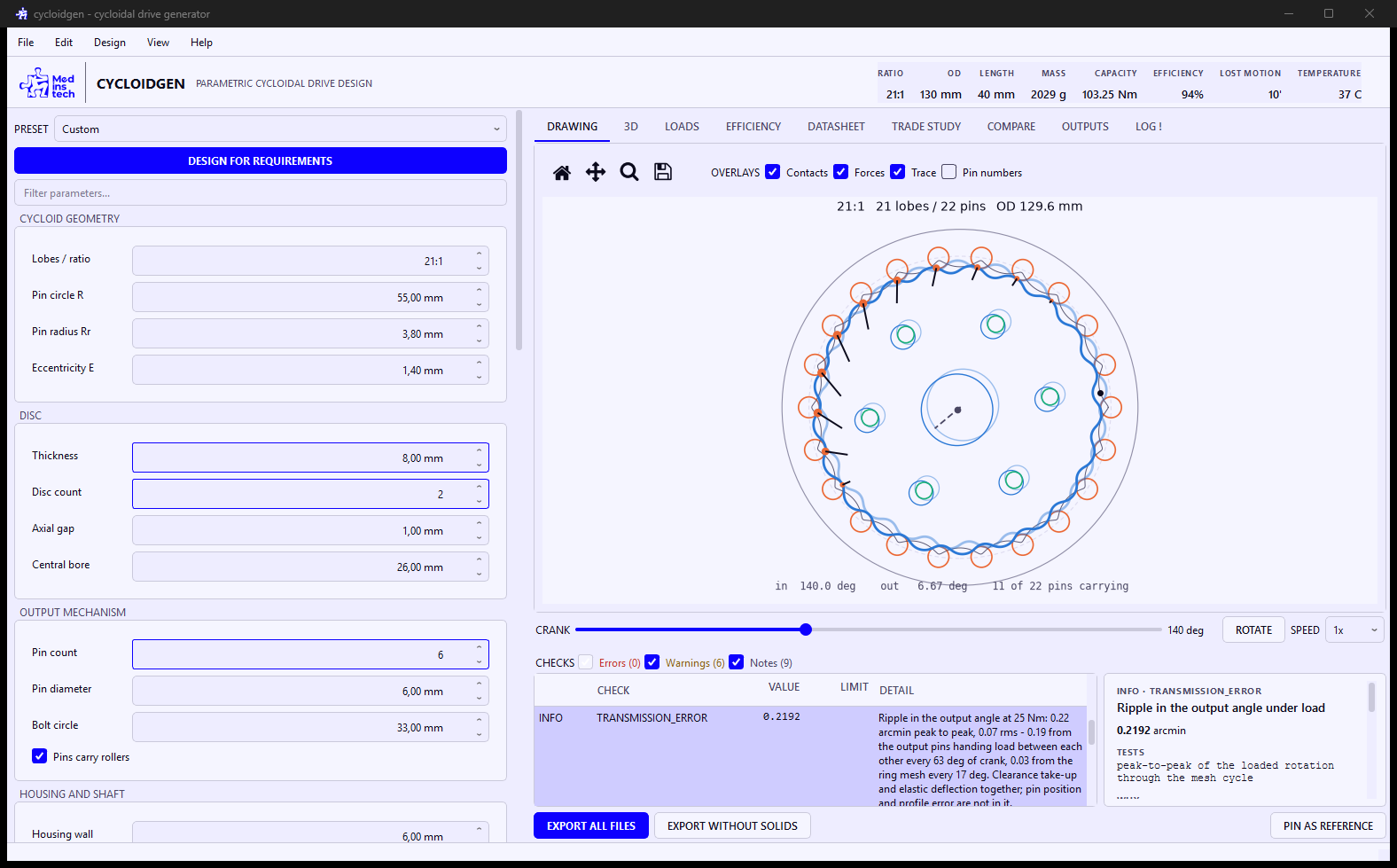
Selecting a check tells you what it tests, why it matters and what to change;
the parameters it names light up in the panel on the left.

---

• Exact geometry. The conjugate profile in closed form, verified to sit at exactly the pin radius from the pin-centre locus — envelope deviation 0.0 µm.
• A datasheet, not a drawing. Contact stress, torque capacity, efficiency, torsional stiffness, lost motion, transmission error, PV and running temperature, lubrication regime, mass and inertia, bearing life.
• Fifty-five checks that explain themselves. Each says what it tests, what goes wrong physically when it fails, and which parameter to move — and lights that parameter up in the panel.
• Requirements in, geometry out. Say ratio, torque, speed and envelope; get a shortlist that passes every check, with the trade-offs side by side.
• Nothing is asserted that is not verified. 771 tests, and where two parts of the app describe the same gearbox they are checked against each other — the 3D mesh against the volume the exported solid encloses, the export manifest against the files that land on disk.

Preliminary sizing numbers, not a certification. See How far to trust the analysis.

Jump to — Run it · Three ways to use it · What it produces · The geometry · What it tells you · Checks · In the app · Tests · Performance · Contributing

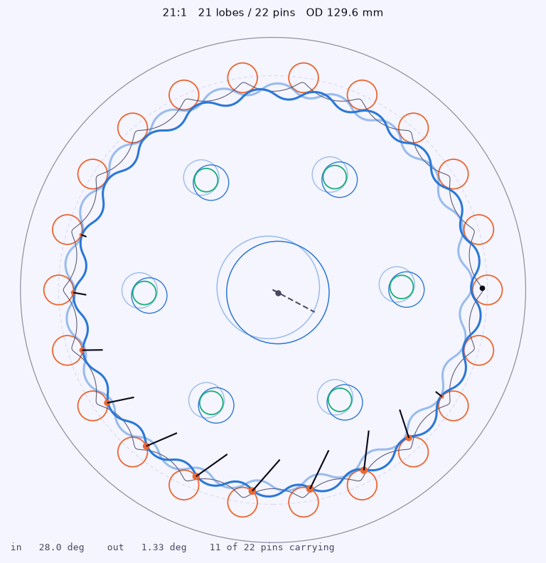
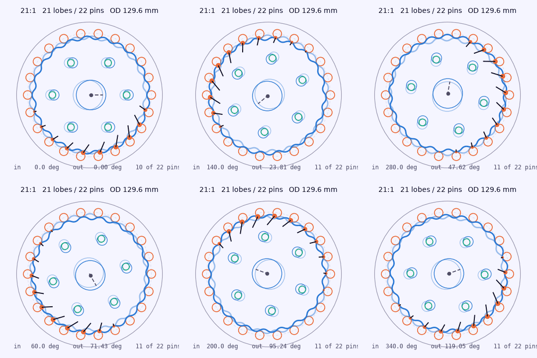
The drawing is a simulation, not an outline. The dots are where the disc touches each ring pin and the arrows are the load it carries there, both off the same kinematics the checks and the datasheet use; the faint wavy ring is the path one point on the disc rim travels over a full output revolution. Twenty-one turns of the input, one of the output.

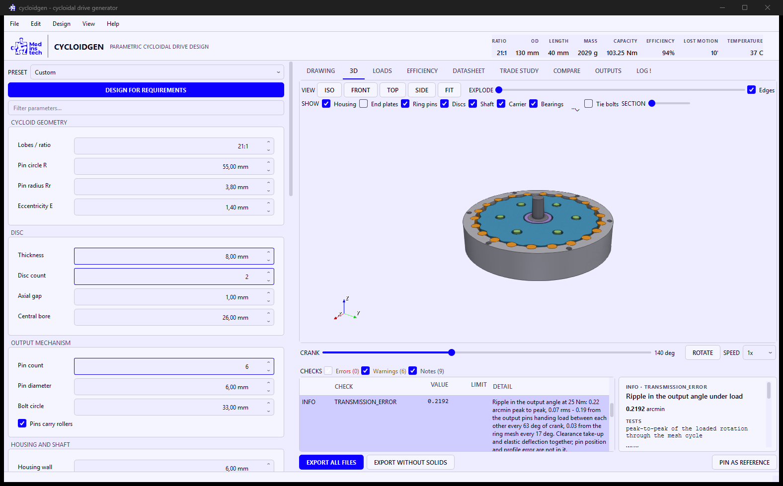
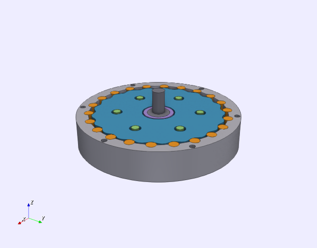
The 3D view turns on the same crank as the drawing, so the mechanism is the same mechanism in both. It is built from the same closed-form profile — not tessellated from the exported solids — so it cannot drift from what you get in the STEP file, and it still works in a build with the CAD kernel stripped out.

That second picture is the viewport itself, cropped out of the running window rather than redrawn. On a machine with no OpenGL the same scene comes out of a software painter instead, which is what the PDF report embeds.

Run it

Python 3.10 – 3.12, on Windows, Linux or macOS.

pip install cycloidgen
cycloidgen

That is the whole thing, window and all, on all three platforms. It is a large install — most of a gigabyte, nearly all of it Qt and the OCCT CAD kernel — so a virtual environment is worth the two extra lines.

There is also a build that needs no Python at all, on the releases page: a Windows installer, and a Linux AppImage — one file, chmod +x, double-click. The installer is unsigned, so SmartScreen will want a More info ▸ Run anyway; see RELEASING.md. If the AppImage will not start, the machine is missing FUSE 2 — either install it (libfuse2 on Debian and Ubuntu) or run the file with --appimage-extract-and-run, which unpacks it and needs nothing.

To work on it rather than with it, install the checkout in place:

py -3.12 -m venv .venv                          # Windows
.venv\Scripts\python -m pip install -e ".[dev]"
.venv\Scripts\python -m cycloidgen

python3 -m venv .venv                           # Linux, macOS
.venv/bin/python -m pip install -e ".[dev]"
.venv/bin/python -m cycloidgen

Headless, without opening the window:

python -m cycloidgen --ratio 29 --out ./my_gearbox
python -m cycloidgen --design saved.json --out ./x --no-solids
python -m cycloidgen --ratio 29 --no-cam-bearing --no-shaft-bearings --out ./x

Or put a whole grid of designs through it and get a table rather than a folder of parts — every combination, every number, for a spreadsheet or a fitting script:

python -m cycloidgen --ratio 21 \
    --vary lubricant="None (dry)" \
    --vary lubricant="Grease NLGI 2 (EP, moly)" \
    --vary surface_roughness_um=0.2:12:8 \
    --csv study.csv

--vary repeats: twice for one field is two values of one axis, once each for two fields is a grid. Numeric fields also take lo:hi:steps. Designs that fail a check stay in the table with their error codes, because where the feasible region ends is most of what a study is for. Without --csv it prints a summary instead.

Or state what you need and let it find the geometry:

python -m cycloidgen --optimise --ratio 29 --torque 20 --rpm 1500 \
    --max-od 120 --process "CNC machined" \
    --disc-material "Steel 4140 (hardened)" --rollers --out ./x

Three ways to use it

Give it a design. Set the twenty-odd parameters and the app tells you what is wrong with them — this is the original mode and everything below still applies to it.

Give it requirements. Ratio, torque, speed, envelope, process, materials, and what to optimise for; the search returns a shortlist of geometries that pass every check, with the trade-offs side by side. Ctrl+R in the app, or --optimise on the command line.

Give it a grid, or call it from Python. --vary puts a design through every combination of whatever you name and returns a table. The analysis underneath is an ordinary importable library — no display, no Qt, no matplotlib — and docs/api.md is what it looks like from the outside: the spec, the analysis, the exporters, the sweep, the grid and the search, with every example in it executed by the test suite so it cannot go stale.

Nine free dimensions is too many to grid, so most of them are derived from the relationships good cycloidal geometry actually obeys — eccentricity from the shortening coefficient, pin radius from the undercut limit, bore from the shaft, bolt circle as a fraction of the band that is genuinely available. What is left is six continuous knobs and two discrete ones, screened in closed form before anything expensive runs. A search that finds nothing reports why: 1,400 of 1,500 candidates were over your diameter limit is a usable answer, an empty list is not.

What it produces

Four groups, chosen together or separately — in the app's Outputs tab, on the command line with --only, or with the two quick export buttons.

File	Group	Contents
disc.dxf	drawings	Drawing of the whole drive: disc profile as a closed LWPOLYLINE sampled to the chord tolerance, plus bore, output holes, ring pins and housing, on separate layers
disc.svg	drawings	Same drawing, 1 unit = 1 mm
dxf/	drawings	One cutting file per part — each disc on its own, the ring plate, a carrier drilling template drilled for the press fit rather than for the disc's running hole, and the two end plates with their tie-bolt circle and motor pattern
assembly.step	solids	Full gearbox: housing and its two end plates, ring pins, phased discs, eccentric shaft, output flange with its bearing boss, every bearing that fits, coloured
step/	solids	Each part as its own solid, in its own frame
stl/	solids	Each part separately — STL has no assembly structure. A multi-disc stack gets disc_1.stl, disc_2.stl, … because the discs are not the same part (see below)
bom.csv	data	Every part: quantity, material, size, mass, make or buy, and the bearing designations the sizing study picked
report.json	data	Every parameter, derived value, load, stiffness, temperature, mass and finding as plain data
report.pdf	data	Drawing and 3D view, geometry, checks, contact stress, stiffness and backlash, PV and temperature, mass, bill of materials, bearings, and an exploded build order
motion.gif	animation	The drive turning, looping, with contacts and contact forces — for a document, a chat or an issue. See below for why it loops without a jump

The Outputs tab lists all of that for the current design before anything is written — every file by name, what it is for, and where it will land — then fills in the sizes afterwards and opens any of them on a double-click. The same list is available headlessly:

python -m cycloidgen --ratio 29 --list-outputs
python -m cycloidgen --ratio 29 --only drawings,data --out ./x

That list is not a second copy of the truth. cycloidgen/export/manifest.py declares every deliverable once; write_bundle, the Outputs tab and --list-outputs all read it, and a test compares the declaration against the files that actually appear on disk — including this table.

Every file says which build wrote it. A saved design, the JSON report, the PDF and every DXF carry the version, because none of the numbers here are measurements: they are a model's answers, and the model gets better between releases. So a design saved by an earlier build says so when you open it — which quantities may have moved, and that the inputs still mean what they meant — instead of quietly reporting a different mass than the one you wrote down. RELEASING.md says which version digits are allowed to move a number and which one is defined as the digit that cannot.

Why the animation loops without a jump. A GIF restarts whether or not the mechanism is back where it started, and one that is not reads as a fault in the drive rather than in the file. Different parts close at different times. The disc, the ring contacts and the force arrows close after a single input turn — one turn walks the disc on by exactly one lobe pitch, and a profile with N lobes is unchanged by that rotation. The output carrier does not: it advances 360/N per input turn and repeats every 360/output_pin_count, so it needs N / gcd(N, output_pin_count) turns — five for the 15:1 preset, seven for the 21:1, fifty-nine for the 59:1. When the exact period does not fit the frame budget the answer is not as many turns as will fit: any whole turn leaves the disc closed, so the run to choose is the one whose carrier lands closest to a hole pitch, and at 29:1 that is five turns (2.1° out) rather than ten (4.1°).

Making that true of the pixels rather than only of the arithmetic took two fixes, both of which are improvements in their own right. The chord-tolerance sample count is now rounded up onto a whole number of samples per lobe, so the sampled polygon has the disc's own symmetry instead of sampling each lobe from a slightly different place. And the disc outline is drawn as a closed path rather than a polyline with its first point repeated, so its seam is a join like any other — a seam travels round the rim as the disc turns, and it was changing a handful of pixels every frame at a place where nothing was happening.

The geometry

With R the ring-pin circle radius, Rr the pin radius, E the eccentricity, N the lobe count, Np = N+1 pins and K1 = E*Np/R:

D(t) = sqrt(1 + K1² − 2·K1·cos(N·t))
x(t) =  R·cos(t) − E·cos(Np·t) − Rr·(cos(t) − K1·cos(Np·t)) / D(t)
y(t) = −R·sin(t) + E·sin(Np·t) + Rr·(sin(t) − K1·sin(Np·t)) / D(t)

The reduction is the lobe count, i = N = Np − 1, and the output pin holes are the pin diameter plus twice the eccentricity.

Sign warning. The equivalent psi formulation needs a leading minus: psi(t) = -atan2(sin(N·t), R/(E·Np) - cos(N·t)). The positive-sign variant is widespread online and is wrong - it deviates by millimetres and the disc interferes with the pins by about 1 mm, which seizes the drive. tests/test_profile.py pins both the correct form and the trap.

Everything above is verified numerically rather than trusted:

• Envelope property - every profile point sits exactly Rr from the pin-centre locus (deviation 0.0000 µm). This is what makes the disc roll instead of dig in.
• Meshing sweep - a full input revolution runs with under 2 µm residual interference, while a ratio one tooth away jams by 450-730 µm. That proves the profile and the motion law together.
• Undercut limit - Rr < 1/max(-kappa) of the locus. The locus curvature collapses to (A + B·u)/(C − D·u)^1.5 with u = cos(N·t), so the extreme is a closed-form root rather than a 40 000-point scan — which is what makes the design search affordable. Cross-checked against the brute-force result.
• Assembly fit - every output pin stays inside its hole through a full revolution, on every disc; the disc clears the housing bore.

Clearance: which way the offset goes

Both clearance levers have to shrink the disc. It reaches R − Rr + E from its own centre, so growing the generating roller (equidistant) and shrinking the generating pin circle (pin_circle) each pull the profile inward. Two of the three modes originally had the pin-circle sign backwards and cut a ~200 µm interference instead of a clearance; both cancelled itself out to almost exactly zero. Nothing noticed, because every other test ran on the default mode.

So the clearance is no longer assumed — it is measured, as the distance from each pin centre to the manufactured profile less the pin radius (core.kinematics.mesh_gaps). PROFILE_INTERFERENCE is an error and CLEARANCE_NOT_DELIVERED a warning, and every mode is tested to open a real gap.

That measured gap then feeds the load model, which answers the question the old README could only flag as a limitation:

• an equidistant offset gives every pin the same normal gap, so a contact only comes into mesh once the disc has turned far enough to close it. Contacts with a short moment arm need much more rotation than the long ones — so at low torque a handful of pins carry everything, and the peak force is several times the ideal share. Capacity is derated accordingly.
• more torque pulls more pins in; a tighter process pulls more pins in. Both are visible in the datasheet as pins carrying load, and both are tested.

Multi-disc stacks: the discs are different parts

A disc sitting on crank phase p has to rotate by p/N to stay meshed with the ring. But every disc is coupled to the same output carrier, so every disc must also share the carrier's rotation. Both can only hold if each disc's output-hole pattern is turned back against its lobes by -p/N.

So in a two-disc drive the second disc is the first one with its holes moved half a lobe pitch. They are not interchangeable — swapping them jams the drive. They would only be identical with 2*N output pins, which is normally far too many, and the app tells you (DISCS_DIFFER) when that is not the case. The per-part files, the STLs and the bill of materials all keep them apart.

This was wrong in the first version and is now pinned by tests/test_assembly.py. The visible symptom is worth knowing: in the drawing, the green output pin must stay inside its blue hole at every crank angle. When it pokes out, the hole pattern is at the wrong angle.

What it tells you

Beyond the geometry checks, every design gets a datasheet:

• Torque capacity, both on the ideal load share and derated for what clearance actually does to it.
• Torsional stiffness in Nm/arcmin and lost motion in arcmin, from Hertzian line-contact springs (Johnson's elastic approach) on the ring and output stages, in series with the parts they are mounted in — the ring pin seats, the carrier pins in bending, the carrier plate, the disc body, the housing barrel and the input shaft. Every one of those is reported on its own line, because "everything else" as a single number is a number to distrust, and because on most designs the softest part is a surprise. On a printed drive the two halves are comparable, which already costs the answer a third. The better the mesh, the worse the imbalance: a ground steel drive stiffens its contacts by two orders of magnitude and its cantilevered carrier pins by nothing at all, and ends up an order of magnitude softer than its own mesh.
• Transmission error — the ripple in output angle under a steady load, which is the number that decides whether a drive can position. Lost motion is the play before the output moves; this is what it does once it is moving, as the mesh hands load from one contact to the next. Each stage is swept over its own period, and they are not the same: the output stage repeats every 2·pi·N/(n·(N−1)) of crank, about two and a half lobe pitches, and measuring it over a lobe pitch instead reports about half the ripple that is there. A phased disc stack cancels much of it — the discs ride opposite halves of the same cycle — which a stiffness average cannot see, because phasing leaves the mean alone and only moves the ripple.
• What your tolerance costs. Everything else in the app places the pins exactly, and with a uniform clearance that means they all come into mesh together. Enter the true position your shop holds and the load sharing is solved over a batch of rings drawn from that tolerance zone — a single number does not say where each pin went, worst case is a ring nobody will build, and nominal is a ring nobody has built. Out comes the middle ring and the bad one: stiffness, load concentration, lost motion and transmission error, each with its tail. Past the point where the tolerance approaches the clearance the pins interfere and the drive binds, and the app says so rather than quietly reading an interfering pin as a free preload.
• PV and running temperature. PV is the wear limit, and it is what actually finishes a printed drive — a PLA disc can sit well inside its stress allowable and still wear round in an afternoon. Quoted on the projected-area convention the published limits use, not the Hertzian peak; the two differ by several times and are not interchangeable.
• Mass, inertia, unbalance. Off the real lobed section, not a cylinder. Reflected inertia at the input, and the shaking force a single disc throws — which goes as the square of speed. Evenly phased discs cancel the force and leave a couple.
• Disc web stress. The ligament beside the output holes is the thinnest structural member in the drive and nothing else was looking at it.

Checks

Fifty-five of them. Errors block export; warnings do not; several are readings rather than tests.

Profile — K1_TOO_HIGH · K1_HIGH · UNDERCUT · UNDERCUT_MARGIN · PROFILE_SELF_INTERSECT · PROFILE_INTERFERENCE · CLEARANCE_NOT_DELIVERED · PIN_RADIUS_SUGGESTION

Layout — PIN_OVERLAP · PIN_SPACING · HOLE_HITS_BORE · HOLE_BREAKS_RIM · THIN_INNER_WEB · THIN_OUTER_WEB · OUTPUT_HOLES_OVERLAP · OUTPUT_HOLE_SPACING · ECCENTRIC_TIGHT · DISCS_DIFFER

Manufacturing — CLEARANCE_DEFICIT · HOLE_CLEARANCE_DEFICIT · TOOL_RADIUS · PIN_POSITION

Load and stress — PRESSURE_ANGLE · HERTZ_STRESS_RING · HERTZ_STRESS_MARGIN · HERTZ_STRESS_OUTPUT · LOAD_CONCENTRATION · WEB_SHEAR · WEB_SHEAR_MARGIN · FATIGUE_LIFE · FATIGUE_MARGIN · FATIGUE_NOT_MODELLED

Precision — TORSIONAL_STIFFNESS · STRUCTURAL_COMPLIANCE · LOST_MOTION · TRANSMISSION_ERROR

Wear, heat and life — LOW_EFFICIENCY · LUBRICATION_REGIME · PV_LIMIT_RING · PV_MARGIN_RING · PV_LIMIT_OUTPUT · PV_LIMIT_CAM · OVERTEMP · RUNNING_HOT · SHORT_BEARING_LIFE · NO_BEARING_FITS · BEARING_DOES_NOT_FIT · BEARINGS_OMITTED

Mounting — HOUSING_BOLT_CLASH · MOTOR_SHAFT_MISMATCH · MOTOR_FACE_CLASH · MOTOR_RADIAL_LOAD

Dynamics and mass — SINGLE_DISC_UNBALANCE · UNBALANCE_FORCE · MASS

Selecting a check in the app highlights the parameters it is actually about, so you are not left guessing which of twenty-odd numbers it wants you to change. That list is not maintained by hand: the codes are parsed out of the calls that raise them, and a check added without an explanation fails the suite.

PIN_RADIUS_SUGGESTION is worth knowing about: the equivalent contact radius works out to R_eq = Rr·(1 − Rr/rho_c), a parabola peaking at Rr = rho_c/2. Contact stress is therefore lowest at half the critical pin radius, and the app suggests it.

In the app

• Drawing — the live 2D simulation. A crank slider and playback at a chosen speed, and four overlays that can be turned on independently: contact points sized by the share of load they carry, contact forces to scale, the traced path of a point on the disc rim, and ring pin numbers. Input and output angles are read out under the drawing, so the reduction is something you watch rather than something you are told. A pinned reference design shows underneath as a ghost outline.

  

  Everything drawn comes off core.kinematics, the module that was verified against a full-revolution meshing simulation — the picture cannot tell a different story from the datasheet. Force arrows are scaled against the worst force over a whole lobe pitch rather than against the current frame, so an arrow that grows means the load grew and not that the scale moved under it.

  That animation is a file the app writes, not a screen recording: seven input turns of the 21:1 preset, which is exactly its period.

• 3D — the assembled drive on the same crank. Drag to orbit, right-drag to pan, wheel to zoom, standard viewpoints, an explode slider, per-group visibility so you can take the housing off and watch the mesh — the tab opens with the end plates already off, because with them on the assembled view is a closed cylinder with a shaft out of one end — and a capped section plane — the cut reads as solid material with the cut faces a shade darker, not as a hollow casting. Turning Edges on draws the part's features — rims, hole lips, the join between a cylinder and its end — and not the triangulation underneath them.

  The bearings are in there too, at the size the sizing study picked rather than the size of the space they go in — a ring on the cam inside each disc bore, sleeves over the ring and output pins where a roller was selected, and the two shaft supports where the end plates belong. Where a bearing is not drawn it is because the model has nothing for it to sit in, and its note in the schedule says which case it is.

  They also switch off one at a time, from the … beside the group: they sit in four different places, and looking at the cam bearing down its bore means putting the others away rather than putting all of them away.

  Mounting says how it bolts to the world. Pick a motor frame and the input end plate gets that frame's register and bolt pattern — a square for a NEMA, because four holes on a circle of the same size land where the motor has nothing — and the app checks the three things that pairing can get wrong: a motor whose shaft is not the shaft the drive was drawn around, a pattern that falls into the bore or off the rim, and, when you have chosen to let the motor carry the crank, whether its own bearings are up to it. The output end of this topology is a boss on the axis rather than a bolt face, so what it needs is somewhere for a coupling to grip; it now stands proud of the plate instead of coming out flush.

  That is the picture. Whether the drive actually has them, and which ones, is a design decision, under Bearings in the parameter panel. Each seat can be left on auto — the smallest catalogue part that fits it and lasts the life you ask for — or given a designation, which is what you want when a bearing you already own is doing the deciding. A named part is checked against its seat and never quietly swapped for one that fits; if it will not go in, the check names the dimension that is wrong and the 3D view leaves it out rather than drawing it shrunk to size.

  Three of the five load paths can also be built without a bearing at all, and plenty of drives are. Switching one off takes the part out of the schedule, the BOM, the STEP and the 3D view, and changes the physics with it: a drive with no cam bearing runs its disc bore straight on the cam, which grows to fill it, and pays the sliding coefficient at the fastest contact in the machine. The load path stays on the schedule either way, saying what is carrying it instead — a motor's own bearings do not stop the crank reaction existing.

  

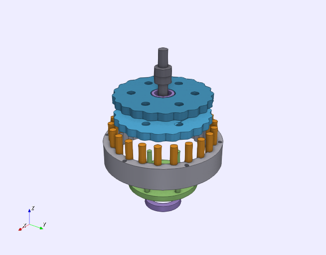
  It renders on the GPU through VTK — which costs no new dependency, because the CAD kernel that writes your STEP files already brings it. Depth buffer, smooth shading off feature-angle normals so the pins are round rather than faceted, a three-point light rig, screen-space ambient occlusion sized off the drive so a pin sits in its pocket, and multisampled edges. Geometry is uploaded once per design; turning the crank sets one transform per part, so a frame is bounded by the display's refresh rate and a 59:1 drive with sixty pins costs exactly what a 15:1 one does.

  There is a software fallback — the same scene, back-face culled and painted back to front with QPainter — for a build with the kernel stripped out, a machine with no OpenGL, or a remote session that will not forward it. A flat-shaded gearbox beats a tab that shows an error. It is also what draws the 3D views in the PDF, where a vector figure is worth more than a screenshot, and what makes the projection testable on a machine with no display at all.

  macOS gets a different viewport, not a different renderer. VTK's own Qt widget builds its GL context directly on the view winId() returns, with WA_PaintOnScreen set — an attribute Qt documents as X11-only, on a platform whose views have been layer-backed and mandatorily so since 10.14. The first render blocks the main thread as the tab opens and takes the application with it, and because that is a process dying rather than an exception, the fallback cannot catch it and step in. So macOS runs a widget of our own over vtkGenericOpenGLRenderWindow, rendering inside the context Qt already owns — no second context, no native handle to get wrong. CYCLOIDGEN_VTK_QTGL selects that backend either way; CYCLOIDGEN_VTK=0 drops any machine back to the software painter, and is the first thing to try if the 3D tab misbehaves.

  The mesh is verified against the volume of the solid that gets exported, part by part, so the picture and the STEP file are the same gearbox.

• Outputs — every file an export writes, by name, with what it is for and where it will land, before anything is written. Sizes fill in afterwards and a double-click opens any of them.

• File ▸ Export animation (Ctrl+Shift+E) writes whichever view you are looking at as a looping GIF — the drawing with the overlays you have ticked, or the assembly from the angle, explode and part visibility you have set. It renders off the GUI thread with a real progress bar and a Cancel that leaves no half-written file, and it uses the appearance you are in rather than the print surface the bundled motion.gif gets.

• Loads, Efficiency, and a Datasheet tab with everything above.

• Trade study — sweep any one parameter and watch torque capacity, efficiency, lost motion and mass move together, on their own real units, with the infeasible band shaded rather than silently dropped.

  

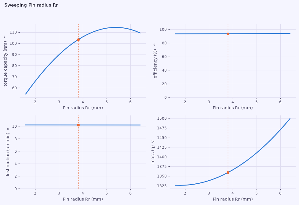
  Read off that chart: pin radius buys torque capacity up to a genuine optimum and then gives it back — the PIN_RADIUS_SUGGESTION check in closed form — while costing mass the whole way and doing essentially nothing for efficiency or backlash. Note the flat panels start at zero. A quantity that moves by a tenth of a percent gets an axis that says so, rather than one scaled to make the noise look like a decision.

• Compare — pin a design, change things, and see exactly what moved and by how much. Running the optimiser pins the design it replaced automatically.

• Appearance follows the desktop and can be overridden per user (View ▸ Appearance). Both palettes are contrast-tested rather than asserted, and chrome and figures switch together — a chart on a white slab inside a dark window is the thing following the desktop theme was meant to prevent. The light mode is tinted paper, mixed from the brand's own blue, rather than white; the PDF still prints on white, because a tint on every figure is ink someone pays for and gains nothing on paper.

  Structure is drawn rather than implied by shadow, and the brand blue is spent only where it means this one — the primary action, the focused field, the selected row and tab, a ticked box. It used to be on every group heading, tab and rule as well, and at that point it stops being emphasis.

• Checks filter — severity toggles carrying their own counts, because a design routinely produces a dozen findings of which ten are notes and the two that block an export sit somewhere in the middle.

• Units (View ▸ Units) — millimetres or decimal inches, for everything you read: the parameter fields, the datasheet, the checks list, the comparison table and the drawing's own title. Everything you hand over stays millimetres — DXF, STEP, STL, the JSON report and the PDF — because a CAD file whose units follow a preference is a CAD file nobody can trust. Internally the design is millimetres and never leaves them: a switch reloads the widgets from the spec rather than converting what is in them, so toggling the menu twenty times cannot move a number.

• Explain this check — select a finding and the panel beside it says what the check tests (the relation, in the notation above), what goes wrong physically when it fails, what to change and in which direction, and how many times clear of the limit you are. The parameters it names are highlighted in the panel at the same time. cycloidgen/core/explain.py declares one explanation per check code; a test parses the source for the calls that raise codes, so a check cannot be added without one or left behind when it goes.

• Log — everything the app would otherwise print to a terminal you do not have. Checks as they appear and clear, searches with their shortlists, sweeps, exports, plus every Python warning, stray stderr write, and any exception that escapes a worker thread. Timestamped, level-filtered, copyable. The tab marks itself when something arrives while you are looking elsewhere. It earned its keep immediately: the first run surfaced a RuntimeWarning from a negative log term in the contact-stiffness solver that had been silently producing NaNs on degenerate geometry.

• Undo/redo, recent files, a parameter filter box, and the session reopens on the design, tab, crank angle and panel split you left. The split is stored as a proportion: remembering pixels hands a narrower screen most of its width to the parameter panel. The analysis runs off the GUI thread with generation numbering, so a slow result can never overwrite a newer one.

Preferences live wherever the platform puts them, or in a file of your choosing via CYCLOIDGEN_SETTINGS — which is what makes a portable install possible, and what lets the test suite run without rearranging your actual application.

How far to trust the analysis

The ideal load model treats the disc as rigid and each contact as a linear spring, so force is proportional to moment arm and only the pushing half of the pins carries load — the classical Kudryavtsev/Lehmann assumption. The stiffness model does see clearance and is what the capacity derating comes from, and it counts the parts around the mesh rather than calling them rigid — but it counts them as ideal parts. Joints, fits and fasteners are not in it, so a real drive measures softer again, and two of the six terms rest on an assumption the geometry does not settle (see analysis/compliance.py, which states both). Pin position error is modelled only if you enter a tolerance; with none entered the ring is perfect, which no ring is. Transmission error is the drive's own share only — clearance take-up and deflection, both of which it solves; pin position error, profile error and runout are the manufacturing half and are not modelled, so a real drive measures worse. The thermal model is a single lumped body in still air with no conduction into whatever the gearbox is bolted to. Bearing catalogue values are nominal metric-series figures. PV limits are dry-against-steel design-guide values. The lubrication model builds a Dowson-Hamrock film for a line contact and applies it to the two conforming ones as well, where the formula was not derived — their film is capped at the radial clearance, which is a real bound rather than a fitted one, but a close-fitting journal is properly a hydrodynamic problem and this is not that. Starvation, grease channelling and the transient film at start-up are not modelled, and all three make it worse, so a contact it places in the boundary regime is there.

These are preliminary sizing numbers, not a certification. Calibrate against a physical prototype before committing to a design.

Layout

cycloidgen/
├── units.py    what lengths are *shown* in; everything inside is millimetres
├── core/       spec (the one source of truth), profile, kinematics, validate,
│               explain (what each check tests, why, and what to change),
│               guide (what each parameter is and how to choose it)
├── analysis/   mechanics (Hertz), stiffness (contacts, backlash, transmission
│               error), compliance (the parts around the mesh, as springs),
│               tolerance (where the pins actually are), lubrication (the
│               film, and the friction it earns), thermal, mass, efficiency,
│               bearings
├── design/     optimise (requirements -> geometry), sweep (trade studies)
├── viz/        3D geometry and rendering maths, no Qt: mesh, scene (the
│               software projection), vtkbridge (mesh -> VTK polydata)
├── export/     manifest (what a bundle contains), dxf, svg, solid (OCCT),
│               bom, animation (the looping GIF)
├── report/     plots (shared by UI and PDF), build
└── ui/         PySide6 window, 3D viewer, outputs tab, declarative field table,
                optimiser dialog, trade-study tab, undo/redo history, log panel,
                branding (palette and stylesheet), plotbar (the trimmed
                matplotlib toolbar)
tests/          771 tests; the envelope, pin-in-hole, clearance-sign,
                mesh-versus-solid and animation-closes tests matter most

Two boundaries in there are load-bearing. core and viz do not import Qt, which is what lets the geometry and the renderer be tested without a display and what keeps one piece of code drawing both the window and the PDF. And export/manifest.py declares every output file exactly once — the writer, the Outputs tab, --list-outputs and the table above all read it.

Tests

.venv\Scripts\python -m pytest -q

569 tests, about 300 s. Most of that is CadQuery writing solids; the pure analysis tests run in a few seconds. The Qt tests run headless (QT_QPA_PLATFORM=offscreen, set by the test modules themselves) and redirect preferences into a temporary file, so the suite cannot rearrange your own application.

Two of them are worth calling out because they are the ones that keep separate representations of the same gearbox honest:

• The 3D mesh against the exported solid. Every part's mesh volume is computed by the divergence theorem and compared against what OCCT says the STEP body encloses, to within faceting error. The same test checks that each part is a closed surface — the vector areas of its faces must cancel exactly, which catches a missing end cap, a wall built for the wrong number of edges, or a loop wound the wrong way round. It has already earned its keep: it found the eccentric shaft double-counting the barrel inside its own cams.
• The manifest against the disk. An export is compared against what the manifest promised — exactly those files and no others — including the table in this README.

CI runs ruff, then the suite on Linux, Windows and macOS across the oldest and newest supported Python, then separately exports a full bundle and runs a design search from the command line — the tests cover the pieces, that job proves the whole thing still runs end to end.

Lint rules live in pyproject.toml so they mean the same thing locally and in CI. ruff format is deliberately not part of it: the repository has a hand-aligned style the formatter would rewrite wholesale, and a lint that hunts bug shapes is worth more than one that enforces a preference.

The README figures come out of the same plotting code the app and the PDF use, so they cannot drift from what it actually draws:

.venv\Scripts\python docs\make_figures.py

The two screenshots of the window are taken by a second script, and it needs a real desktop session rather than the offscreen platform the tests use — twice over. Offscreen Qt has no fonts, so every label renders as tofu; and the 3D tab's viewport is a native OpenGL surface that QWidget.grab composites around, leaving a black hole where the gearbox was. So the window is opened, driven — hero design, overlays on, a check selected, the camera set — and photographed through PrintWindow with PW_RENDERFULLCONTENT, which asks Windows for the window's own rendering including native children and does not care what is stacked on top of it:

.venv\Scripts\python tools\make_screenshots.py

Performance

A full re-analysis is about 110 ms — every check, every load, the stiffness model, transmission error and the whole datasheet, on each parameter edit. It was 106 ms when it did a fraction of that work, and three things bought the room the rest of it went into: the mesh sweep is computed once and shared instead of three modules each running their own, the profile, the undercut limit and the measured mesh clearances are cached, and the self-intersection test uses a uniform-grid broad phase instead of sampling every other segment against all the rest — which was also skipping over crossings it should have caught.

Entering a pin position tolerance is the one thing that costs real time, about half a second, because it stops analysing a gearbox and starts analysing a batch of them. It is off unless you ask for it.

Animation runs on a 33 ms tick and both views fit inside it. The drawing costs about 10 ms a frame, down from 25: the artists are built when the design changes and repositioned when the angle does, so a crank move no longer rebuilds a couple of hundred patches and re-runs tight_layout. The 3D view sets seven transforms and hands them to the card, so it is bounded by vsync rather than by us; the software fallback does the whole projection in numpy in about 1 ms and spends the rest painting, for roughly 13 ms a frame.

Neither view is redrawn while its tab is hidden — a hidden matplotlib canvas will still honour draw_idle with a full render, which is ten milliseconds a frame spent on something nobody can see — and neither rebuilds geometry for a change that did not touch it. The mesh cache is keyed on the fields the geometry actually depends on, so changing a material or the rated torque does not send a fresh copy of the assembly to the graphics card. That key is a hand-written list and therefore a liability, so a test perturbs every field of GearSpec in turn and requires that an unchanged key really does mean an unchanged mesh.

The live animation loops over the mechanism's own period, which is lobes input revolutions — one output revolution — and not one turn of the crank. After a single input turn the disc and the carrier have moved on by 360/lobes and are not back where they started, which is what used to put a visible jump in the loop every four seconds. The exported animation cannot afford that many turns at a legible frame rate and picks its run differently — see Why the animation loops without a jump above.

Standalone build and installer

Three artefacts come out of a release, and they are not alternatives:

	who it is for	platforms
Installer (.exe)	somebody who wants to run the app and does not have Python	Windows
AppImage	the same person, on Linux	x86-64, glibc 2.35 and up
Wheel on PyPI	anybody with Python 3.10 – 3.12; also the only way to import cycloidgen	Windows, Linux, macOS, x86-64 and arm64

There is no cross-platform installer format, so the first two are separate programs doing the same job by opposite means. NSIS writes an installer that unpacks the bundle into Program Files and registers it; an AppImage installs nothing — it is the bundle, in a squashfs image behind a small runtime that mounts it. macOS has neither yet: pip install is the answer there, and an unsigned .dmg would be a worse experience than that rather than a better one.

.\packaging\release.ps1                        # lint, tests, bundle, installer
.\packaging\release.ps1 -FastPack -SkipTests    # quick internal build

python -m PyInstaller cycloidgen.spec --noconfirm   # Linux
bash packaging/appimage.sh                          # -> releases/*.AppImage

Or the two steps by hand:

.venv\Scripts\python -m PyInstaller cycloidgen.spec --noconfirm
dist\cycloidgen\cycloidgen.exe                         # the window
dist\cycloidgen\cycloidgen-cli.exe --list-outputs      # the command line
makensis /INPUTCHARSET UTF8 packaging\cycloidgen.nsi   # needs NSIS 3.x

The Windows bundle carries two executables over one analysis, which is the pythonw.exe / python.exe arrangement and for the same reason. cycloidgen.exe is windowed — it is what the shortcuts point at, and a console build there put a black window behind the application every time somebody opened it from the Start menu. cycloidgen-cli.exe is the console one, for headless runs. A single windowed build would have taken the command line away and taken it away badly: a frozen windowed process has no stdout at all, so --version would not print nothing, it would raise.

The AppImage carries one. console is a Windows subsystem flag — a field in the PE header saying whether the loader allocates a console — and Linux has no equivalent; every process gets whatever streams it was handed. A second binary there would not be a second behaviour, only a second copy of the same one under a name implying a difference that does not exist.

The installer upgrades in place — it clears the previous version first, because unpacking a PyInstaller bundle over another one leaves modules and DLLs from the old version that load in preference to the new ones and then fail in ways that look like an application bug. It waits if the application is running, registers properly with Add/Remove Programs, and leaves your preferences and last design alone when uninstalled. English and Turkish.

Versions come from one line in cycloidgen/__init__.py: the wheel, the About box, the executable's file properties, the installer's filename and the release workflow all read that one, and tests/test_version.py fails if a second copy appears or if the changelog has no section for it. See RELEASING.md.

Verified working, GUI and CLI, including STEP/STL export. Two things about the PyInstaller spec are load-bearing and easy to break:

• The entry point is launcher.py, not cycloidgen/__main__.py. PyInstaller runs its entry script as a top-level module, which breaks relative imports.
• _casadi.pyd (pulled in by CadQuery's assembly solver) gets relocated to the bundle root while the DLLs it links against stay in casadi/, so the spec copies those DLLs to the root as well. Without it the exe dies with DLL load failed while importing _casadi.

The bundle is about 1.2 GB, essentially all OCCT. If that matters, build with --no-solids in mind: the drawings-and-report path does not need CadQuery, and dropping cadquery, OCP, casadi and vtkmodules from the spec cuts the bundle to a fraction of the size.

Where it is going

One thing is worth more than everything else on the list: calibration against real hardware. Every number here is a first-principles estimate with a stated model and stated limits. That is honest, and it is also the ceiling — the moment there is a table of predicted versus measured, this stops being a calculator and becomes a calibrated instrument.

The half of that which was not waiting on a lathe is in: fitting the model's free constants against measurements is a script over a grid, and the grid, the importable analysis and the documented API are all here now.

After that, in rough order: bearing life under combined load and misalignment; and more kinds of drive — compound and multi-stage, RV-type, a pinwheel output. On the output side, dimensioned drawing sheets with tolerances and a title block, which is what a shop actually wants; 3MF with per-part colour; STEP AP242 with PMI. Open an issue if one of those is what stands between you and using it — that moves it up the list.

Contributing

CONTRIBUTING.md covers setup, the house style, the settled questions, and what a change looks like here. The short version: numbers are verified rather than asserted, comments say why, and ruff format is deliberately not part of the build.

The most valuable contribution needs no code at all — build one of these and measure it.

Also: CHANGELOG.md · RELEASING.md · SECURITY.md · CODE_OF_CONDUCT.md

License

Apache-2.0. Copyright 2026 Medinstech. See LICENSE.

The Medinstech name and logos under cycloidgen/ui/assets/ are trademarks and are not covered by that licence — see NOTICE. They load through a single module (cycloidgen/ui/branding.py) so that replacing them in a fork is one obvious change.

The numbers this produces are preliminary sizing estimates, not a certification — see How far to trust the analysis above. Apache-2.0 disclaims warranty for a reason, and that disclaimer is meant literally here: validate against a physical prototype before anything load-bearing depends on it.