In this mini-project, used as a demonstration of quick use of OpenCV for a Python course I am (at the time of writing) running, we explore Image Saliency Detection.
Saliency Detection is the process where image processing and computer vision algorithms are used to locate the most "salient" regions of an image. What does this mean? Well, saliency is defined as "the quality of being particularly noticeable or important" i.e. the prominent parts of an image, in this case. Our brains and visual systems (eyes), through evolutionary processes, have adapted to rapidly (and rather unconsciously) focus on the most important regions within our visual field. Applying this to computer vision, it allows our systems to pick out key parts of a static image, or video sequence. Use cases of this include the cameras on many cars that pick up road signs, updating the driver of the latest speed limit in force - for example.
Applications of saliency detection may also be applied to other aspects of computer vision and image processing including:
- Object Detection: Rather than using the somewhat brute-force approach classically deployed (sliding window and image pyramid), only apply the (admittedly computationally expensive) detection algorithm to the image's most salient regions. More salient regions should hopefully be more likely to have objects present.
- Advertising and Marketing: Apply techniques to validate design logos and advertisements intended to "stand out" and "pop" from a quick or passing glance.
- Robotics: Design robotics and potentially autonomous systems with visual / environmental recognition systems similar to our own.
- Static Saliency: Relies on image features and statistics to focus and localise on the most prominent image regions.
- Motion Saliency: Typically these rely on video or frame-by-frame input data. Frames are processed, tracking objects that appear to "move", with these considered salient.
- Objectness Saliency: Saliency Detection algorithms computing "objectness" generate a set of "proposals" - these are fundamentally just 'bounding boxes' of where objects are thought to exist within an image.
Bear in mind - object detection is not the same as computing saliency.
The SD algorithm has no idea if the image contains an object of a given type, or not. Rather, it reports areas where it "thinks" objects reside within, meaning other processing systems (such as humans, or other algorithms) are responsible for classifying and making any decisions based on this classification/prediction. One benefit of SDs are their speed - useful for real-time applications where we wouldn't be able, or want, to run computationally expensive algorithms over all pixels in all image frames.
We can check if the saliency module has been installed by opening a Python shell and trying to import it...
$ python
>>> import cv2
>>> cv2.saliency
<module 'cv2.saliency'>Code for this section can be found in static_saliency.py.
NB: Static Saliency Method here comes from Montabone and Soto's 2010 work
Required packages include argparse and of course OpenCV.
First, the code imports the desired image (as specified in the command line argument). Then, using the cv2.saliency module and calling the StaticSaliencySpectralResidual_create() method, a static spectral residual saliency object is instantiated. We then invoke the computeSaliency method and pass in our image. As a result, we produce a saliencyMap, namely a floating point grayscale image highlighting the most prominent salient regions of the image. Floating point values in this case are ∈[0,1] with values closer to 1 being "interesting" and those closer to 0 being "not so interesting".
Now, as I'm sure you've worked out by now, images aren't displayed in the range x ∈[0,1], rather they use the range x ∈[0,255] (for 8-bit images). Therefore, we scale the image values to do this and then display both.
NB: Fine Grained Static Saliency Method, coming from Hou and Zhang's 2007 CVPR paper
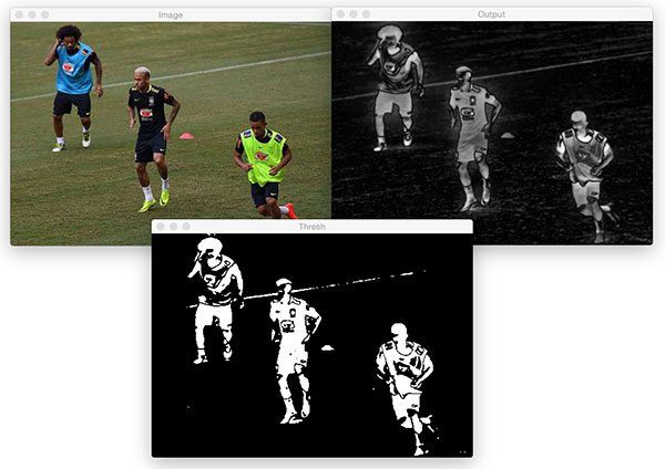
This second sub-method begins entirely the same as our first one above, with the exception that we're choosing to create a more fine-grained object. Also, we'll perform a threshold to demonstrate a binary map that we could perhaps process for contours. This may be used to extract each salient region, for example.
Using the StaticSaliencyFineGrained_create() method we instantiate the fine grained static saliency object, before then again computing our saliencyMap. OpenCV has been implemented in differing ways for fine-grained vs. spectral saliency. This time, we already have scaled values in the range x ∈[0,255] so we can display the image as processed. Then, our method computes a binary threshold image to help find likely object region contours.
Beyond the processing reached above in this method, one might choose to perform a series of erosions and dilations morphological operations prior to finding and extracting contours. This hasn't been undertaken in this mini-project, but may serve to be an extension in future.
For the first method, we see below the chosen input image consisting of a motoryacht close to the shore during the daytime. There are reflections, varied surfaces and textures, and other complex details.
 Having applied the algorithm described in the First Algorithm above, we see the image below being produced, which is a Spectral Saliency image of a fairly poor level of fidelity and clarity. This evidently isn't performing well, although it's clear where our object (the motoryacht) is, within the image as it's noticeably higher intensity (per pixel) than the other image regions.
 Extending beyond the initial algorithm we see an improvement when deploying the Fine Grained static saliency detector, with far clearer depiction of our object, and other image details throughout. Reflections in the windows of the boat are distinguishable in this saliency map image, really showing the granularity off.
 Finally, our object is shown below in the thresholded image very clearly, as well as the secondary region of potential interest (namely, the cliffs behind the boat). Using this image as input for an object classifier would be a good starting point if wishing to detect objects such as boats, in a maritime scanning context - using images captured perhaps by another boat as input. The boat in our image takes up a relatively large portion of the field of view, however if taken from afar (by sea or air) it would occupy a significantly smaller percentage of available pixels and, against the ocean/sky view, would need far less processing using this method than alternatives described.

Code for this section can be found in objectness_saliency.py.
First, the necessary packages are imported including numpy, argparse and OpenCV.
The program then loads a given image given as an argument (see below) into memory, before then initialising the objectness saliency detector and establishing the training path. The saliencyMap computation of objectness is then undertaken. As a result, the program is then able to iterate through each detector model, performing in this loop:
- Extract the bounding box coordinates
- Copy image for display purposes and assign a random colour for the bounding box
- Show output image for given detector model
CLI Usage: python objectness_saliency.py [-h] -m MODEL -i IMAGE [-n MAX_DETECTIONS] -d DIFF [-a HERE]

As shown in the above output sample, we see an image of a girl having been processed by the 10 Objectness Saliency Detectors with pseudorandomly coloured bounding boxes highlighting areas deemed to be most likely proposals as mentioned above. Upon inspection, these proposals include areas of the image with the sharpest changes in colour and contour, although the detector sadly does not inform us of the rationale behind proposal selection. Thus, we find this to be a good foundational processor, with these proposals passable to a classifier or other object detection algorithm to make further predictions. Notably, this is less computationally expensive than applying Sliding Windows or Image Pyramids.