An ODE wrapper for RStan which takes a R function representation of an ODE system of equations and generates simulations via RStan. There is also an option to fit data to the ODE system and estimate the initial conditions and/or the parameters.
To clone the repository and build the package locally run the following from R:
devtools::install_github("imadmali/stanode")In this example we simulate an Arenstorf Orbit. For more examples see stan_ode.html
First define the ODE system as an R function (in this example we are using syntax that corresponds to the R package deSolve)
Arenstorf <- function(t, y, p) {
  with(as.list(c(y,p)), {
    D1 <- ((y[1] + mu1)^2 + y[2]^2)^(3/2)
    D2 <- ((y[1] - mu2)^2 + y[2]^2)^(3/2)
    dy1 <- y[3]
    dy2 <- y[4]
    dy3 <- y[1] + 2*y[4] - mu2*(y[1]+mu1)/D1 - mu1*(y[1]-mu2)/D2
    dy4 <- y[2] - 2*y[3] - mu2*y[2]/D1 - mu1*y[2]/D2
    return(list( c(dy1, dy2, dy3, dy4) ))
  })
}
Next specify the initial state values, parameter values, and time steps.
mu1 <- 0.012277471
pars <- c(mu1 = mu1, mu2 = 1 - mu1)
yini <- c(y1 = 0.994, y2 = 0,
          y3 = 0, y4 = -2.00158510637908252240537862224)
time_steps <- seq(from = 0, to = 18, by = 0.01)
Now we can simulate state values from the model at each time step with rstanode::stan_ode.
orbit_rstanode <- stan_ode(Arenstorf,
                           yini,
                           pars,
                           time_steps,
                           integrator = "rk45")
sims <- orbit_rstanode$simulations
To check we also simulate using deSolve::ode.
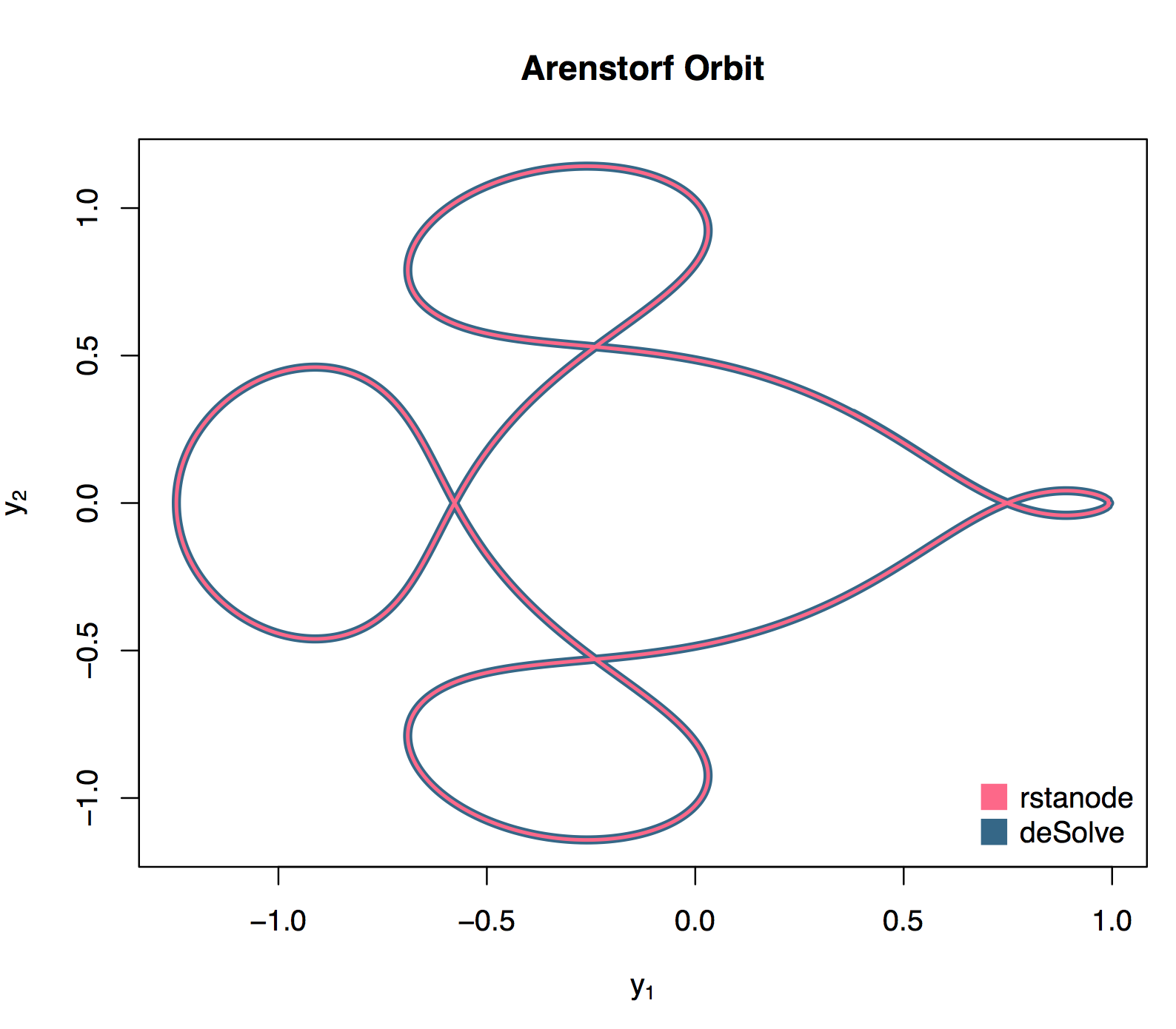
orbit_deSolve <- ode(func = Arenstorf, y = yini, parms = pars, times = time_steps)Overlaying both results for state variable y1 and y2 we have the following plot.
plot(orbit_deSolve[,2], orbit_deSolve[,3], type = "l", col = "#336688", lwd = 5,
     main = "Arenstorf Orbit", xlab = expression(y[1]), ylab = expression(y[2]))
lines(sims[,2], sims[,3], col = "#FF6688", lwd = 2)
legend("bottomright", c("rstanode", "deSolve"), col = c("#FF6688","#336688"),
       pch = c(15,15), pt.cex = 2, bty = "n")