Integrative Analysis Recipe
The Integrative ATAC-seq & RNA-seq Analysis Recipe takes you from bulk RNA-seq and bulk ATAC-seq count matrices to the enrichment analysis of "divergent" genes, identifying those with epigenetic potential versus relative transcriptional abundance. This recipe provides an approach for exploring the relationship between chromatin accessibility and gene expression, supported by unsupervised analyses of the integrated dataset. Specifically, it walks you through the workflow specified in workflow/rules/CorcesINT.smk.
Note
Before you begin, please review our general guide on How to use Recipes and switch your browser to light mode, otherwise you might experience reading difficulties with some of the figures.
Tip
Explore the full interactive report:
This wiki page highlights key analyses, decisions, and results. For more results, explore the complete interactive Snakemake report, where all results specific to this recipe are prefixed with CorcesINT_*.
The term integrative analysis is not strictly defined, but it generally involves combining multiple datasets to uncover insights that a single dataset cannot provide. This can involve different modalities, organisms, or simply many datasets. The goal is to identify both consistencies, which build confidence in the findings (and might increase statistical power) and allow to ask different questions, and discrepancies, which often reveal novel biological mechanisms. The simplest approach is to analyze each dataset separately and then integrate comparable results. For example, one can compare gene-level differential expression statistics from two different RNA-seq experiments or check if the same biological pathways are enriched across matched ATAC-seq and RNA-seq data. For any comparison to be meaningful, the results must share a common comparable feature space.
If this is not feasible or meaningful the "raw" data has to be integrated, which might lead to unforseen complexities and loss of biological information. For integration across modalities, a robust strategy is to map the modality with the larger, more complex feature space (e.g., ATAC-seq genomic consensus regions) to the smaller, more interpretable one (e.g., RNA-seq genes), by quantifying chromatin accessibility across gene-promoters or mapping genomic consensus regions to gene-promoters. Thereby, both datasets become gene-centric, enabling direct comparison.
This recipe demonstrates one such approach where matched multi-omics data are processed together to enable joint statistical testing. By computationally integrating RNA-seq and ATAC-seq data, we can directly model the differences between chromatin accessibility and gene expression. This allows us to systematically identify genes with epigenetic potential (high accessibility but low expression) and those with relative transcriptional abundance (higher expression than expected from accessibility).
Note
Origins of this Method: The concept of epigenetic potential was first introduced by Krausgruber, Fortelny, et al. to demonstrate that non-immune structural cells are epigenetically primed for a rapid immune response under homeostatic conditions. Building on this, Traxler, Reichl, et al. extended the framework by introducing the complementary concept of relative transcriptional abundance. They applied this dual approach to study the dynamics of gene regulation, showing how the relationship between chromatin accessibility and gene expression shifts over time in macrophages during a Listeria infection.
Important
Why: This method moves beyond simple correlation to statistically pinpoint genes where the regulatory relationship is decoupled. It provides a robust framework for discovering genes that are "primed" for future activation or are driven by exceptionally strong regulatory inputs, offering a deeper view into the mechanisms of cell identity and function.
In this tutorial, we aim to integrate chromatin accessibility (ATAC-seq) and gene expression (RNA-seq) data from the human hematopoietic system to uncover regulatory principles that go beyond simple correlation. By re-analyzing the matched datasets from Corces et al. (2016), which we call CorcesINT, we will identify genes where chromatin state and transcriptional output are decoupled. This allows us to systematically map genes with epigenetic potential (high accessibility, low expression) and those with relative transcriptional abundance (high expression relative to accessibility), providing deeper insights into hematopoietic cell fate and function.
Important
Why: While it is often assumed that open chromatin at a gene's promoter leads to high expression, this relationship is not always direct. Identifying genes that deviate from this expectation can reveal key regulatory mechanisms. Genes with high accessibility but low expression may be "primed" for rapid activation, a state we call epigenetic potential. Conversely, genes with higher-than-expected expression may be under the control of other epigenetic mechanisms potent distal enhancers, transcription factors or post-transcriptional regulation, a state we term relative transcriptional abundance. Understanding this interplay is crucial for deciphering the complex regulatory networks that govern cell identity.
At the end of this tutorial, you will have a clear understanding of how to integrate multi-omics data to uncover deeper layers of gene regulation.
To achieve our goal, we combine a series of interconnected MrBiomics Modules into a Recipe. The strategy is to first merge the ATAC-seq and RNA-seq count matrices into a shared feature space. We then computationally integrate the data to remove modality-specific technical differences. Next, we use a specialized differential analysis model to identify genes that diverge between the two modalities. Finally, we interpret these divergent gene sets using enrichment analysis to uncover the underlying biological pathways and potential transcriptional regulators. The recipe is structured as follows(*):
flowchart LR;
    subgraph Data Preparation
        A[RNA-seq counts] --> C{Merge Counts};
        B[ATAC-seq counts] --> C;
    end
    subgraph Integrative Analysis
        C --> D[spilterlize_integrate];
        D --> E[unsupervised_analysis];
        D --> F[dea_limma];
        F --> G[enrichment_analysis];
        D --> H[plot_integration_correlation];
        F --> H;
    end
We use the following MrBiomics modules and one custom script:
- Merge Counts: A custom rule to combine RNA-seq and ATAC-seq promoter counts into a single matrix.
- Split, Filter, Normalize & Integrate: Integrates the two modalities into a common feature space and prepares the data for downstream analysis.
- Unsupervised Analysis: Explores the integrated data structure to ensure successful removal of modality-specific effects.
- Differential Analysis with limma: Identifies statistically significant "divergent" genes between modalities.
- Visualize Correlation: A custom script to visualize the relationship between chromatin accessibility and gene expression and highlight divergent genes.
- Enrichment Analysis: Provides biological interpretation of divergent gene sets using prior knowledge.
Templates of corresponding Methods sections for a scientific publication can be found in each module's README.
Note
Checkpoint: You have reviewed the function of each module by visiting their respective GitHub pages. You should have a conceptual map of how the count data is transformed into biological insight.
(*)The Recipe's real rulegraph visualizes all steps and their dependencies.
A key advantage of this recipe is that it requires no custom coding. The entire analysis is orchestrated through Snakemake using our pre-existing modules and one custom script, with all parameters controlled by simple configuration files.
Important
Prerequisites: This recipe builds upon the results of the RNA-seq Analysis and ATAC-seq Analysis. Ensure you have successfully completed both before proceeding or have matched count matrices (in terms of samples, here cell_type, and features, here gene expression and gene-promoter accessibility, as input. The total disk space required is approximately <1.5GB, and the workflow takes <30 minutes to run on a high-performance computing (HPC) cluster.
The main components are:
-
Main configuration (
config/config.yaml): The central file that points to all other analysis configurations in the sectionCorcesINT. -
Dataset/analysis-specific files (
config/CorcesINT/): A dedicated directory containing all annotation and configuration files for theCorcesINTanalysis. -
Workflow logic (
workflow/rules/CorcesINT.smk): The dedicated Snakemake workflow file that defines the rules and connects the modules. -
Custom script (
workflow/scripts/plot_integration_correlation.R): An R script to generate correlation plots.
Note
Checkpoint: You have located all the configuration, annotation, and Snakemake files mentioned above within the project structure.
This section details each stage of the analysis, explaining the methods, key decisions, and results. We will integrate the previously generated RNA-seq and ATAC-seq data from the Corces hematopoietic dataset.
The first step in any integrative analysis is to establish a common feature space. We achieve this by mapping both RNA-seq and ATAC-seq data to genes. While RNA-seq data is already gene-centric, for ATAC-seq, we use the counts from promoter regions, as generated by the atacseq_pipeline module. A custom rule, CorcesINT_merge_counts, combines the gene-level RNA-seq counts and promoter-level ATAC-seq counts into a single matrix. This merged matrix contains matched samples across both modalities, forming the foundation for our integrative analysis.
Tip
Alternatively, the TSS_counts.csv file can be used in place of the promoter_counts.csv; for details on the differences, please refer to the documentation of the atacseq_pipeline module.
You could do something similar with gene-centric methylation, ChIP-seq, or proteomics data. It's usually best to map to the "smaller" feature space to ensure there's a meaningful overlap.
Note
Checkpoint: The file results/CorcesINT/counts.csv has been created. It contains a single matrix with columns for both RNA-seq and ATAC-seq samples, and rows corresponding to genes.
4.2 • Filtering, Normalization and Integration(!) with spilterlize_integrate
Configuration: config/CorcesINT/CorcesINT_spilterlize_integrate_config.yaml
Annotation: config/CorcesINT/CorcesINT_spilterlize_integrate_annotation.csv
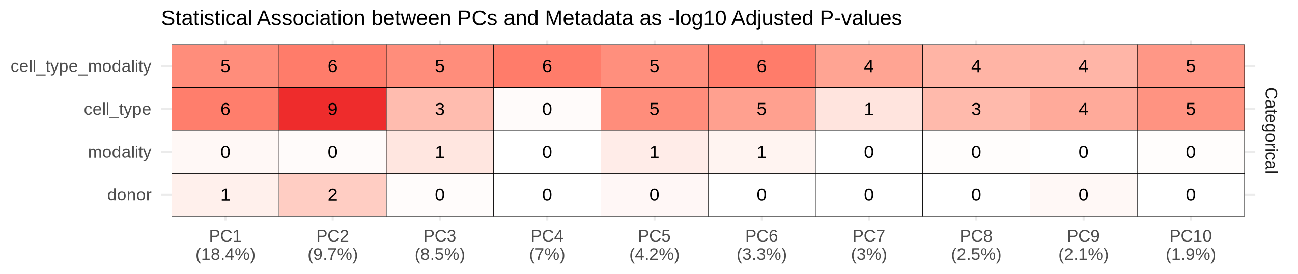
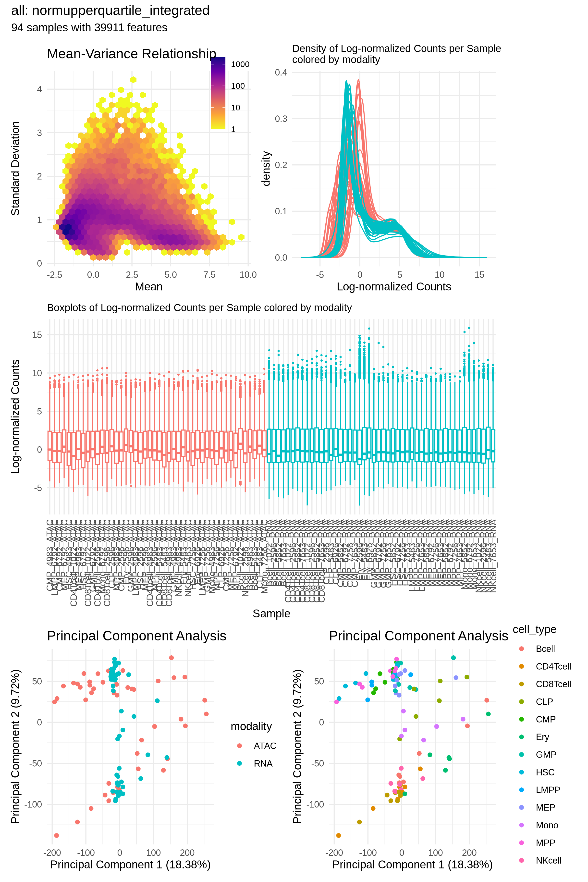
With the merged count matrix, we use the spilterlize_integrate module to computationally harmonize the data. This step is crucial for removing technical differences between the RNA-seq and ATAC-seq assays, allowing for a fair comparison between modalities. For filtering, we define a combined group variable of cell_type and modality. This strategy leverages how filterByExpr works with min.count, ensuring we retain features that are highly abundant in one modality but low or absent in the other within the same cell type—a critical step for identifying divergent genes later. It is crucial to experiment with different normalization methods, as this choice significantly impacts all downstream analyses. Here, upperquartile from edgeR worked best. Following normalization, we use limma's removeBatchEffect function to correct for modality and donor effects, while preserving the biological variation associated with cell_type (i.e., integrate). If covariates, such as donor, aren't removed during integration, you must account for them during downstream modeling. The diagnostic plots clearly show the successful removal of the modality-specific effect, as samples no longer separate by assay type in the PCA. More importantly, the Confounding Factor Analysis (CFA) confirms the success of this approach, showing a clear shift in the dominant source of variation from the technical modality effect to the biological cell_type signal. It is recommended to run multiple experiments with different methods and parameters to find the best integration possible. This is very easy and facilitated by specifying multiple methods in the configuration file.
Important
Why: Direct comparison of raw or separately normalized RNA-seq and ATAC-seq data is misleading due to inherent modality-specific differences in data distribution and scale. By explicitly modeling and removing the modality effect, we create an integrated dataset where remaining differences between assays are more likely to reflect true biology rather than technical artifacts.
filtered |
normupperquartile_integrated |
|---|---|
 |
 |
filtered |
normupperquartile_integrated |
|---|---|
 |
 |
Note
Checkpoint: The integrated data matrix results/CorcesINT/spilterlize_integrate/all/normupperquartile_integrated.csv has been generated. Diagnostic and CFA plots confirm that the modality effect has been successfully removed.
4.3 • Exploratory Data Analysis with unsupervised_analysis
Configuration: config/CorcesINT/CorcesINT_unsupervised_analysis_config.yaml
Annotation: config/CorcesINT/CorcesINT_unsupervised_analysis_annotation.csv
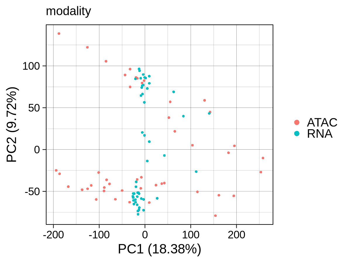
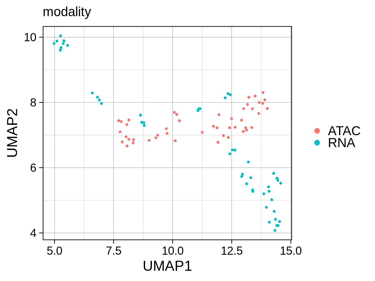
To verify the success of our integration, we apply the unsupervised_analysis module to the integrated data. The PCA shows a clear separation between progenitor and differentiated cells, but a persistent, albeit reduced, separation by modality is still visible. The UMAP reveals a more nuanced structure: while differentiated lymphoid (CLP, B-cells, NK-cells) and erythroid lineages are drawn closely together across modalities, progenitor and myeloid populations still show a noticeable separation by modality. Taken together, PCA exposes residual modality‑specific variance that partially obscures biology, whereas UMAP largely mixes the two modalities and cleanly separates cell‑type clusters along expected hematopoietic trajectories. This indicates that while the integration successfully grouped samples by biological function, significant modality-specific differences remain. This is precisely what our downstream differential analysis aims to capture, providing a strong argument for identifying genes with epigenetic potential and transcriptional abundance.
colored by cell type
|
colored by modality
|
|---|---|
 |
 |
colored by cell_type
|
colored by modality
|
|---|---|
 |
 |
Note
Checkpoint: PCA and UMAP plots in results/CorcesINT/unsupervised_analysis/normupperquartile_integrated/ show clear clustering by cell_type, not modality.
4.4 • Identifying Divergent Genes with dea_limma
Configuration: config/CorcesINT/CorcesINT_dea_limma_config.yaml
Annotation: config/CorcesINT/CorcesINT_dea_limma_annotation.csv
This step is the core of our integrative analysis. We use the dea_limma module in a non-standard way to identify genes where chromatin accessibility and gene expression are divergent based on the integrated data. Instead of comparing biological groups, we use limma-trend with the model ~ 0 + cell_type + cell_type:modality to test for a significant interaction between cell_type and modality, although we removed the modality effect before. This directly asks: "For a given cell type, is the ATAC-seq signal significantly different from the RNA-seq signal, after accounting for baseline differences?"
A significant positive log-fold change (logFC) greater than 1 indicates that ATAC-seq signal is higher than RNA-seq signal, which we define as epigenetic potential (EP). A significant negative logFC less than -1 means RNA-seq signal is higher, which we define as (relative) transcriptional abundance (TA). The results show that as cells differentiate, the correlation between accessibility and expression decreases, and the number of divergent genes increases, suggesting a more complex regulatory landscape in specialized cells. For example, the progenitor HSC exhibits high correlation (0.94) with 2,416 divergent genes, while the differentiated Mono exhibit lower correlation (0.88) with more than twice as many divergent genes (5,090).
Important
Why: This specialized use of differential analysis on integrated data is what allows us to move beyond simple correlation. By statistically testing for the difference between modalities within each cell type, we can robustly identify genes that are primed for activation or are under unusually strong transcriptional control.
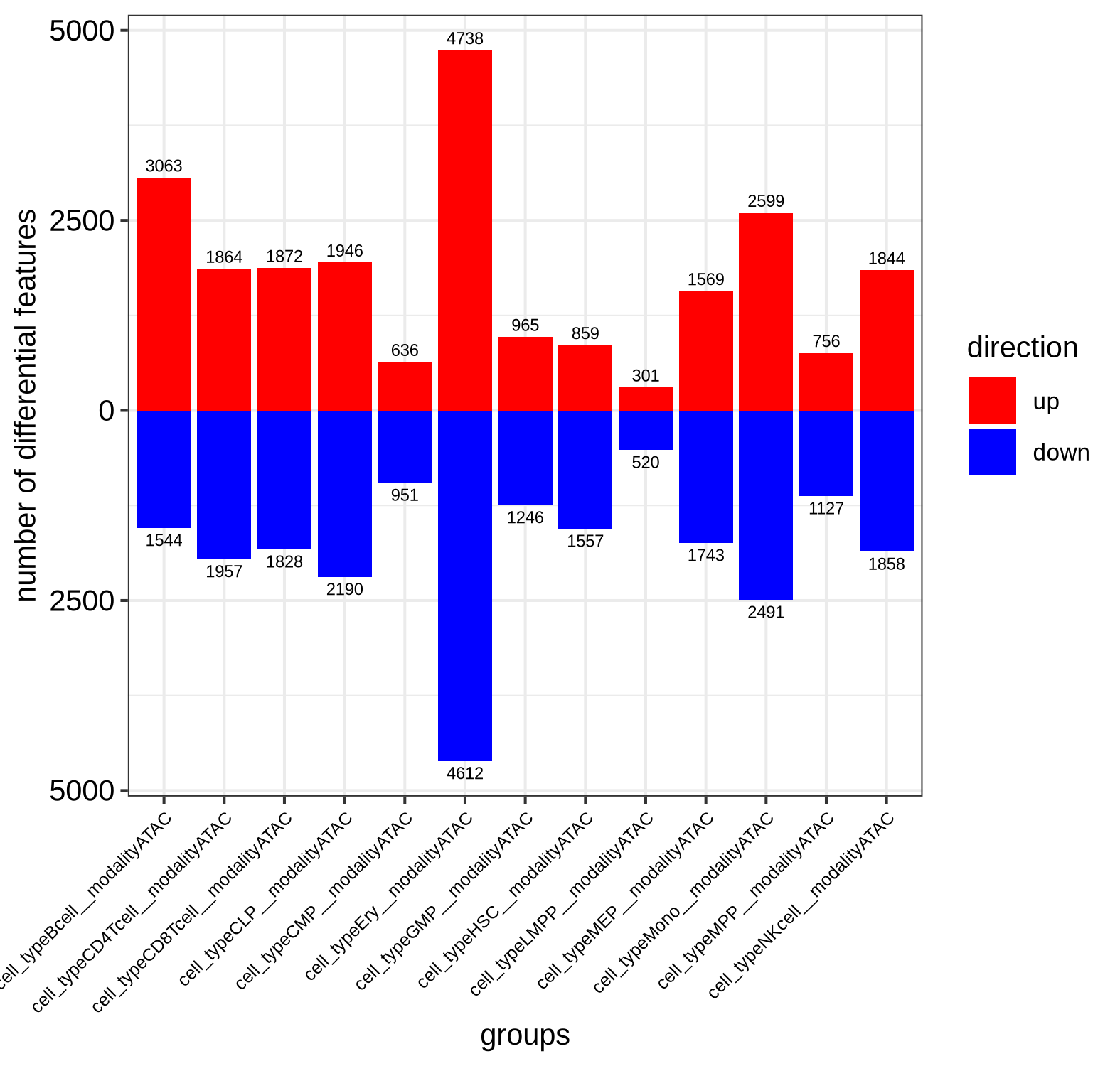
Number of divergent genes per cell type, split by directionality
Tip
Filter Strictly for Divergent Genes: To focus your downstream analysis on the most biologically significant signals, be strict when defining what constitutes a divergent gene. For example, using a higher log-fold change threshold will help isolate only the most pronounced cases of epigenetic potential and transcriptional abundance.
| HSC (progenitor) | Monocytes (differentiated) |
|---|---|
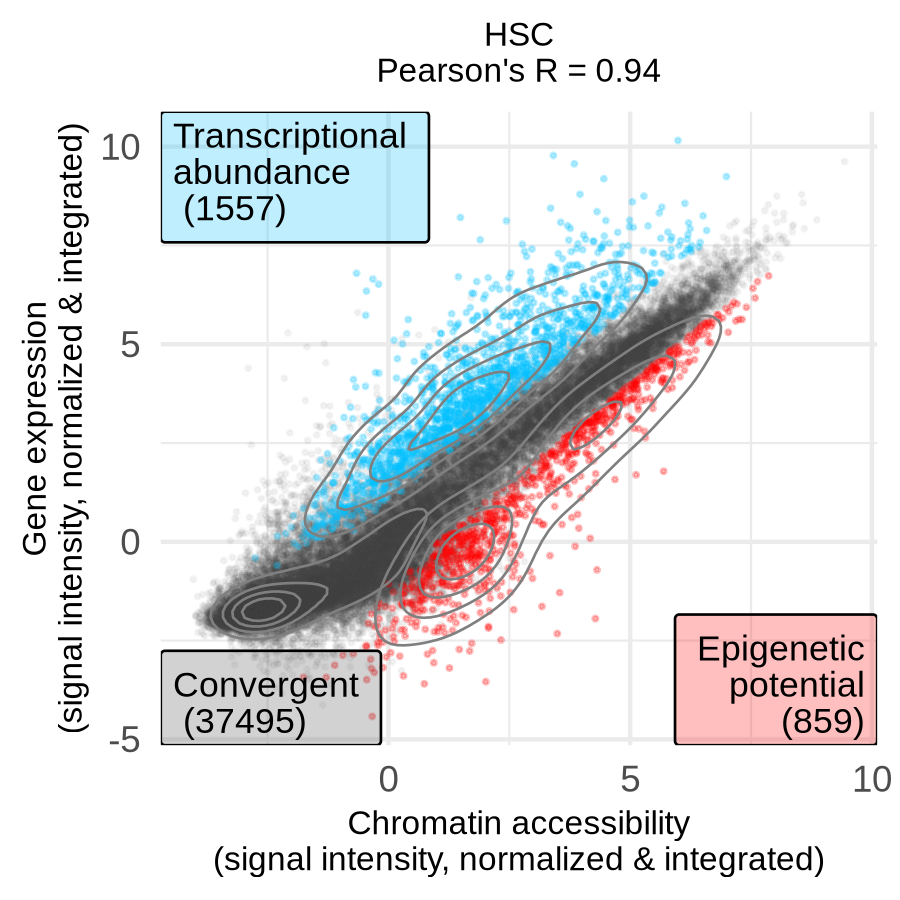 |
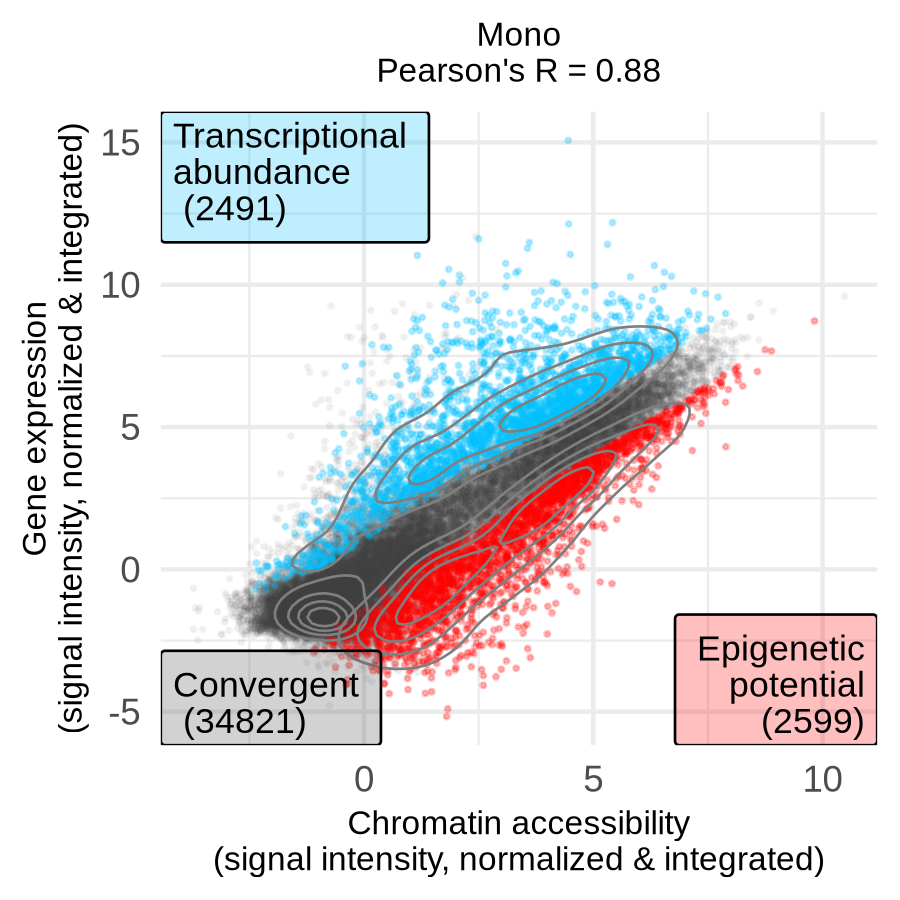 |
Note
Checkpoint: The directory results/CorcesINT/dea_limma/normupperquartile_integrated/feature_lists/ contains files listing genes with epigenetic potential (*_up_features_annot.txt) and transcriptional abundance (*_down_features_annot.txt) for each cell type.
4.5 • Biological Interpretation with enrichment_analysis
Configuration: config/CorcesINT/CorcesINT_enrichment_analysis_config.yaml
Annotation: config/CorcesINT/CorcesINT_enrichment_analysis_annotation.csv
To understand the biological meaning of our divergent gene sets, we use the enrichment_analysis module. We perform pre-ranked Gene Set Enrichment Analysis (GSEA) with GSEApy on the scored differential analysis results. The enrichment results reveal an interesting pattern: proliferative signatures (DNA replication/repair, mitotic checkpoints, translation) exhibit epigenetic potential (red) in CD4Tcell, CD8Tcell, Bcell, Mono, NKcell, HSC and MPP yet equally transcriptional abundance (blue) in Ery, MEP, CMP, GMP, LMPP and CLP, whereas immune‑activation modules such as TNF regulation, B‑cell‑receptor signalling, phagocytosis and neutrophil degranulation invert this polarity, producing a clear reciprocal enrichment across the hematopieitic lineage. This suggests a developmental switch from a state of preparedness to a state of active execution.
| GO Biological Process 2025 | Reactome Pathways |
|---|---|
 |
 |
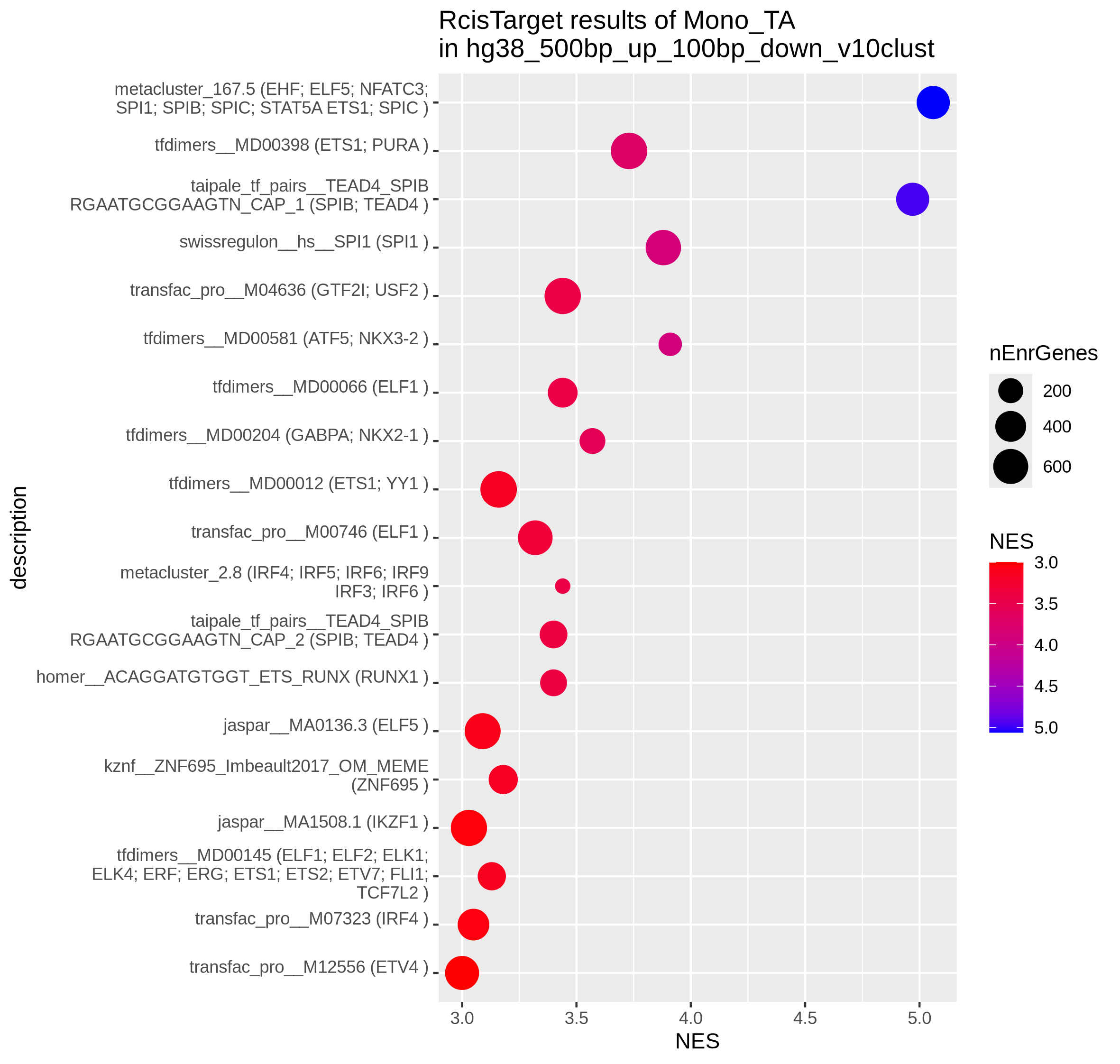
To identify the key transcriptional regulators potentially driving these divergent states, we next performed Transcription Factor Binding Site (TFBS) motif enrichment with Rcistarget on the filtered gene lists of epigenetic potential and transcriptional abundance per cell type. In monocytes the TFBS analysis identified known lineage-specific transcription factors like SPI1, RUNX1 and IRFs enriched at the promoters of genes with transcriptional abundance (TA; right), confirming their role in maintaining cell-type identity and function. On the other hand, genes with epigenetic potential (EP; left) are significantly enriched for binding motifs of the E2F family of transcription factors, which are key regulators of the cell cycle and cell maintenance, further substantiating the observations from previous enrichment results.
| Epigenetic potential (EP) | Transcriptional abundance (TA) |
|---|---|
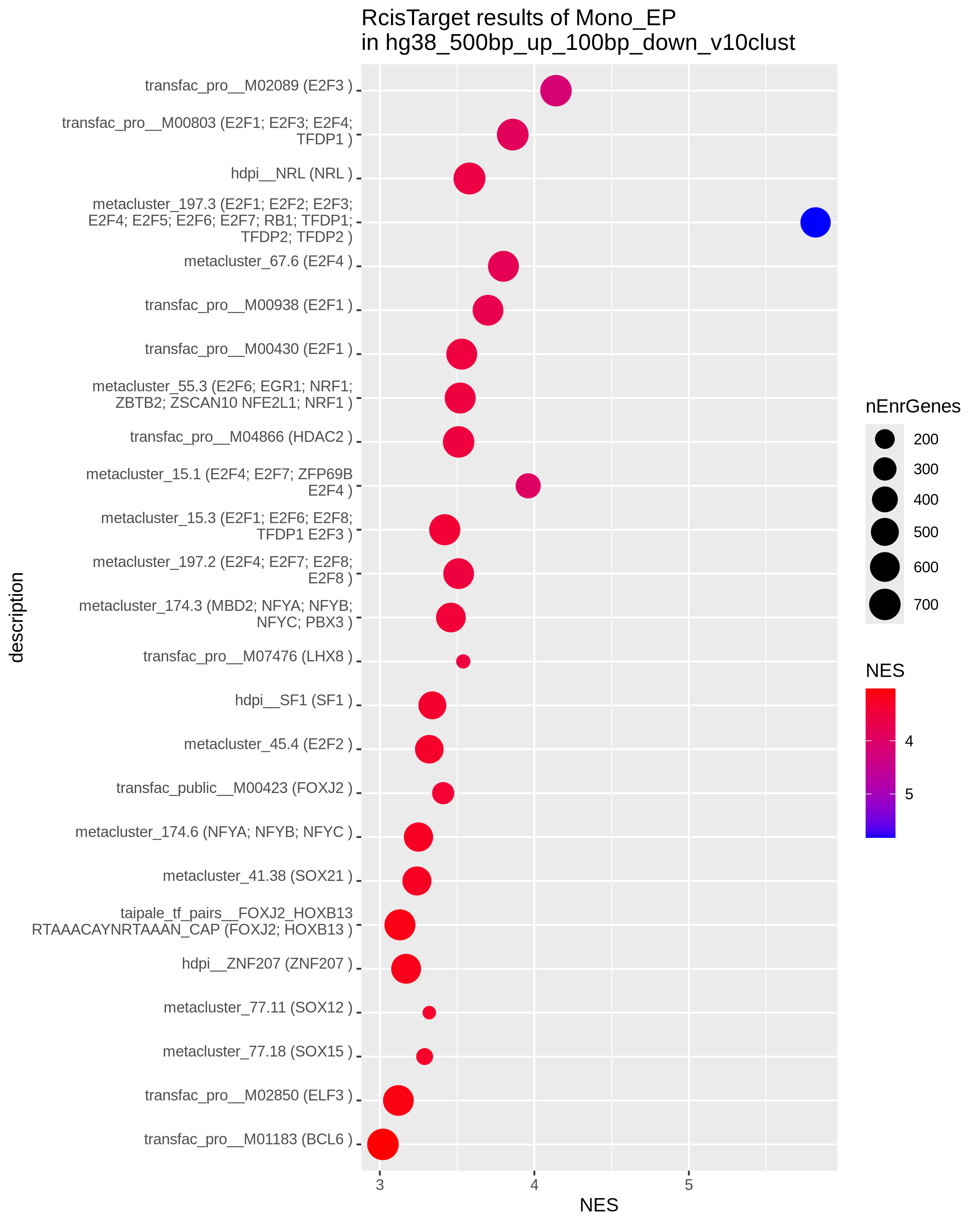 |
 |
Note
Checkpoint: Summary plots in results/CorcesINT/enrichment_analysis/ reveal distinct biological themes for genes with epigenetic potential versus transcriptional abundance, and highlight key transcription factors driving cell-type-specific gene expression programs.
Tip
Iterate with Confidence: This recipe is highly configurable, and experimentation is encouraged. To guide your choices and validate your findings, always use positive controls, such as known marker genes or pathways, as a reference point.
- Incorrect Feature Space Mapping: The entire analysis hinges on correctly mapping ATAC-seq data to a gene-centric feature space (e.g., promoters). Errors here will invalidate all downstream results. Always verify that your promoter definitions are appropriate for your genome and research question.
-
Over-interpretation of Integration: While
removeBatchEffectis powerful, it's not magic. Some residual technical variation may remain. The diagnostic and unsupervised analysis plots are essential for confirming that the biological signal is the dominant source of variation. -
Misinterpretation of the
dea_limmaModel: The differential analysis and limma are used in a non-standard way, by being applied to integrated data and modelling a "removed" effect. It's crucial to remember that the logFC represents the difference between modalities, not a comparison between biological conditions, which we control for usingcell_type. A positive logFC means ATAC > RNA, not that a gene is "up-regulated" in the traditional sense.
Note
Checkpoint: Before starting, double-check your promoter definitions. After each step, critically evaluate the diagnostic plots to ensure the analysis is proceeding as expected.
-
Why not just correlate RNA-seq and ATAC-seq data? Simple correlation can identify broad trends but fails to capture the nuances of gene regulation. It cannot statistically distinguish between genes that are tightly coupled and those that are divergent. Our differential analysis approach provides a robust statistical framework for identifying these important regulatory exceptions.
-
Can this recipe be used for other data types? Yes, the principles can be adapted. For example, you could integrate ChIP-seq data for a specific histone mark with RNA-seq to study the relationship between that mark and transcription. The key is to define a common feature space and a clear biological question that can be framed as a statistical test.
-
What does the decreasing correlation in differentiated cells mean? It is a striking pattern, but be cautious not to over-interpret. One explanation could be that in progenitor cells, the regulatory landscape is relatively simple, and open chromatin is a good predictor of potential expression. In differentiated cells, regulation becomes more complex, involving distal enhancers, complex transcription factor networks, and post-transcriptional control. This leads to a decoupling of promoter accessibility and final mRNA levels, hence the lower correlation.
Important
Feedback, questions, or comments are very welcome, you can reach me via LinkedIn.