A Geobase quickstart blueprint application showing animated ship trails.


This is a React and Geobase application that shows animated ship movements on a map. It uses the powerful PostgreSQL extensions MobilityDb, H3 and PostGIS, all built into Geobase. The application can also interactively query the data to calculate aggregate statistics. With just minimal editing, a user can quickly get started loading, processing and viewing dynamic temporal geospatial data.
AIS stands for Automatic Identification System. It is the location tracking system for sea vessels. It's like GPS but with man additional data fields. There is a dataset already uploaded to Geobase ready for this quickstart. This quickstart will import, processes and make the data available as temporal vector tiles. The vector tiles are then displayed using Deck.gl on a Maplibre map. Users can draw a polygon on the map and the application will display hexagons showing the amount of ship activity in the specified area.
The first step is to have an account on Geobase and to create a new project.
Basic familiarity with Node or running React / Next.js applications (e.g. via nvm and using npm)
Once you're Geobase project is created, you can manually download, clone or create a new GitHub repository using this template by clicking here. This will create a copy of this repo without the git history.
First you will need to load and process the data for the application. You can run SQL from within the Geobase application, or you connect from your own system. Geobase includes a sample of the AIS shipping data in CSV format from 2021 for you to get going quickly. It's probably a good idea to read the SQL to see what it's going to do before you run it.
- Go to the studio
- Navigate to the SQL Editor page
- Click on Geobase Quickstarts
- Select Ship Movement Analysis and review
- Click Run.
See the video below for a quick walkthrough on choosing the quickstart.
select_ship_quickstart.mp4
You can copy the SQL migration file from this repository into a new SQL Query within the Studio.
- Copy the SQL File
- Go to the studio
- Navigate to the SQL Editor page
- Click on New Query
- Paste in the SQL and review
- Click Run.
Locally if you have the PostgreSQL client binaries installed, you can use psql to connect to PostgreSQL on your Geobase server and load in the SQL file.
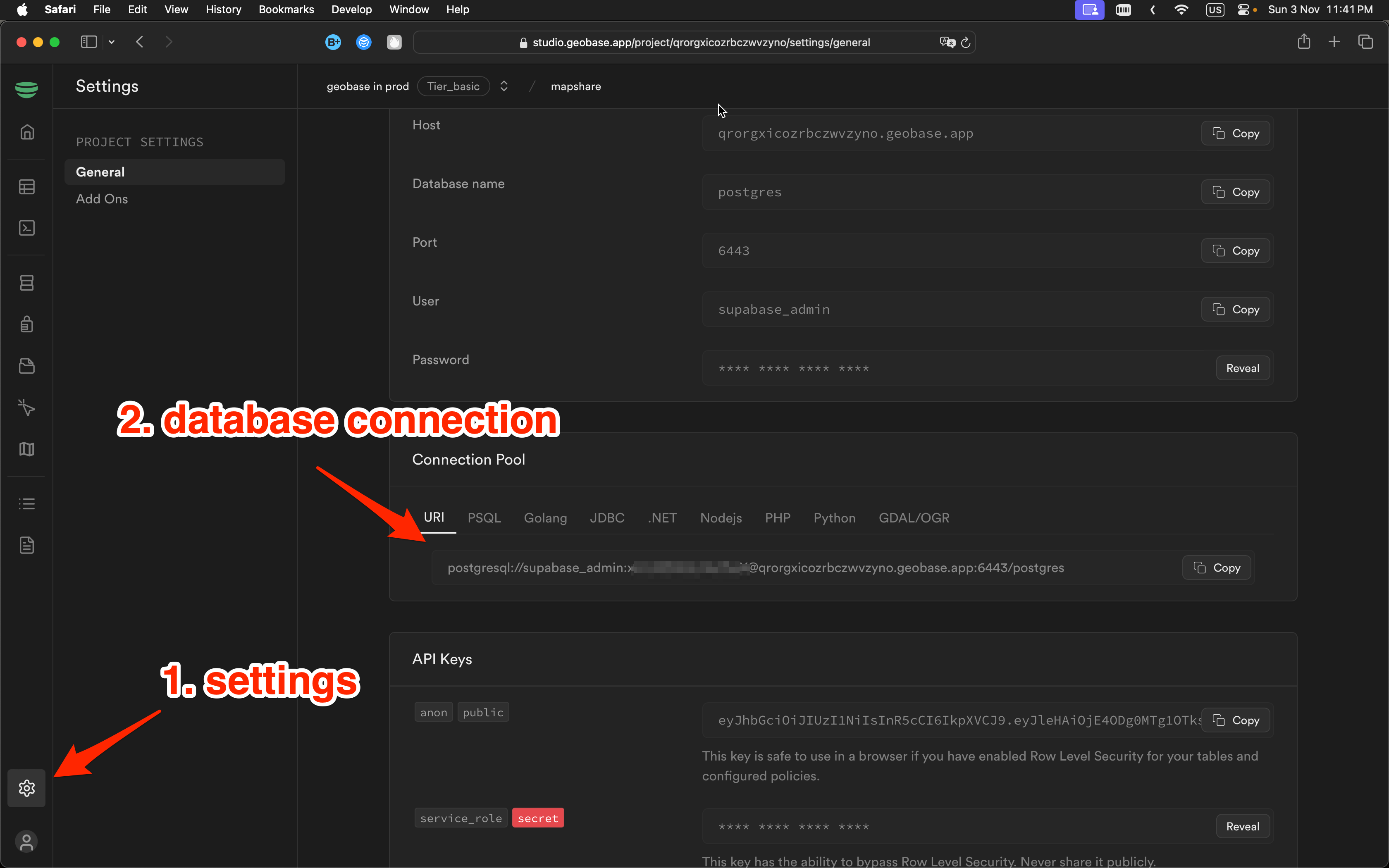
Set the database uri in your environment, you can get it from the Geobase project settings page:
# set the database uri in your environment
DATABASE_URI=<your-database-uri>
psql -d $DATABASE_URI -f geobase/geobase-ship-movement.sqlTo connect your app to Geobase, configure these environment variables. Include them in a .env.local file for local development.
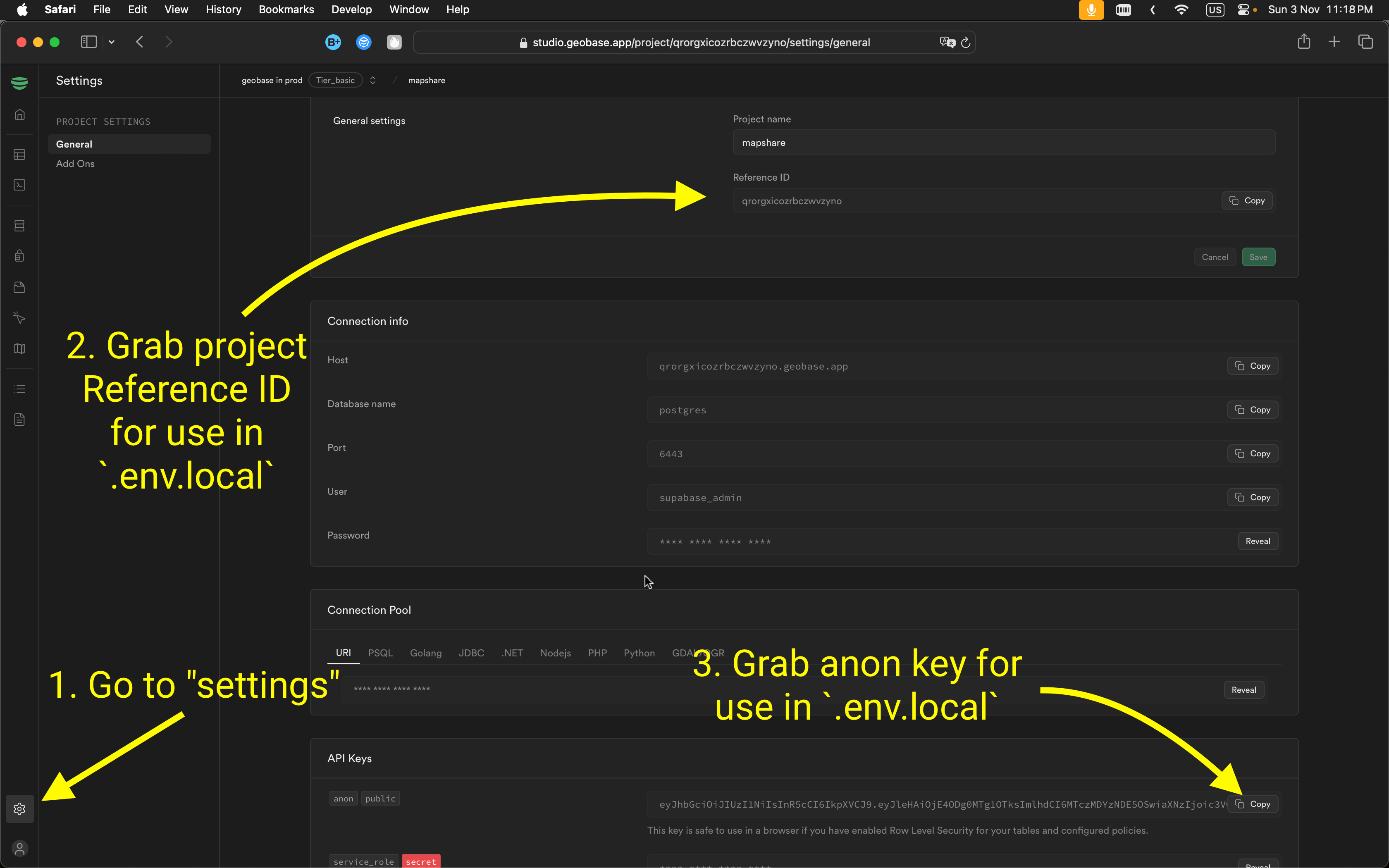
VITE_GEOBASE_URL=https://YOUR_PROJECT_REF.geobase.app
VITE_GEOBASE_ANON_KEY=YOUR_GEOBASE_PROJECT_ANON_KEY
You can find the project ref and anon key in the Geobase project settings page:
``
Use nvm to set node version, e.g.
nvm use 21Install dependencies:
npm install
# or
pnpm install
Run dev:
npm run dev
# or
pnpm run dev
Open http://localhost:5173 with your browser to see the blueprint in action.
You should see something like this animation. Click on the area names to move the map to different areas. "Big Picture" shows the full view. You can start and stop the animation using the timeline control below the map.

You can draw a polygon to query the data to see the activity of the ships as hexagons on the map. Click the "Draw to view activity" button and start drawing a polygon on the map, release the mouse and the hexagons should appear. You can clear these the hexagons by pressing ESC or by clicking the "Clear Hexagons" button.

The easiest way to deploy this blueprint app is to use the Vercel Platform from the creators of Next.js.
Check out the Next.js deployment documentation for more details.
A good summary of how the database is setup can be found in the setup migration file.
The database migration sets up the following tables:
public.AISInput: Raw AIS data imported from the source CSV. Note: This table is dropped after being processed. (590000 rows)public.aisinputfiltered: Filtered AIS data used for analysis. This table is queried by the activity_by_region_and_time_local functionpublic.ships: Data about the ships and their trajectories. Created from the aisinputfiltered table. This table is queried by the ships_fn function. (573 rows)
public.ships_fn(): Create vector tiles (mvt) with embedded timestamps, to be served by the Geobase tile server. This function powers the animated ship movements on the map.public.activity_by_region_and_time_local(): Queries the AIS table with a geoJSON polygon, time interval and map resolution and returns the a timestamp, the h3 hexagon id and count of ship events from the Aisinputfiltered table for that area. This function is used when querying the map by drawing on it.public.get_ships_time_range(): Returns the minimum and maximum timestamps from the ships table. This is used to set the time range for the animation control on the map. You can override this time range data by setting the start_date and end_date in STATIC_TIME_RANGE in thelib/consts.tsfile.
Row Level Security is implemented for the tables to ensure data privacy and access control. As both tables are not going to be directly queried by users and are instead accessed via functions, the quickstart enables RLS on them but with no policies set.
aisinputfiltered, ships:
- RLS enabled, with no policies set.
- Accessed via the two functions (see above)
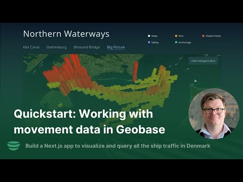
🎥 Take a look at the blueprint overview video on YouTube
For additional information, refer to:
React documentation Geobase documentation
For support, reach out on the Geobase Discord.
The AIS data is from 2021. Historical AIS data is provided by the Danish Maritime Authority. The data shown is a short 3 1/2 hr subset from 1st Aug 2021. This subset, geographically centered around Denmark, contains over half a million rows and records data from a range of vessels, including fishing boats, ferries, yachts under sail, tankers, cargo ships, and even some military vessels.
MobilityDB is an extension of PostgreSQL and PostGIS that provides temporal types, for example a moving vehicle, recording it's speed and position. In this quickstart we use the temporal point type tgeompoint and a sequence of such points creates a tgeompointSeq - conceptually a linestring of temporal points. These points are generated from the AIS dataset by combining the reported latitude and longitude with their respective timestamps.
The mobilityDB functions twavg and speed are used to clean the data to delete ships where there is a large difference between the time weighted average of the reported speed on ground (sog) and the speed of the actual trip. AIS has a certain amount of jitter which is particularly noticeable for stationary ships. To help mitigate this we apply a Douglas Peucker douglasPeuckerSimplify simplification of 3m to the sequences. This not only cleans the data but also reduces its size for maps and speeds up visualizations. There are other simplification methods possible, including minDistSimplify which ensures consecutive values are at least a certain distance apart and maxDistSimplify which removes points that are less than or equal to the distance. Which one you choose for your own projects from depends on the type of data and how you want to visualize it.
A temporal sequence point (tgeompointSeq) represents a continuous movement between spatial positions over time. The function trajectory extracts the spatial path of this movement as a PostGIS linestring trip_geom. The trajectory is used with a spatial index to speed up bounding box intersection queries.
In the ships_fn, we want to include timestamps with our ship line map data. We use the MobilityDB function asMVTGeom to return the line string geometries and times attributes based on the passed in bounds geometry. The ships_fn function also removes ship tracks which are less than 500 meters and to speed up queries does a bounding box overlap operation && of the linestring trajectory of the ship with the requested tile bounds.
Geobase also incorporates H3 support. H3 is a geospatial indexing that uses a hexagonal grid which can be subdivided into progressively finer hexagonal grids. The h3 bindings provide the h3_polygon_to_cells function which identifies the correct H3 hex cells for a user-drawn polygon at a given resolution.
MapLibre is the mapping library used and provides the basemap style.
Deck.gl is a WebGL-powered framework for visual exploratory data analysis of large datasets. It is used with maplibre to render the vector tiles and the animated ship trails on the map.
A vector linestring feature from the tile server has an array of coordinates and a timestamps property. For example:
{
  "type": "Feature",
  "geometry": {
    "type": "LineString",
    "coordinates": [
      [ 15.04302, 54.13267 ],
      [ 15.09658, 53.91566 ],
      [ 15.14739, 53.69995 ],
      [ 15.18173, 53.54438 ]
    ]
  },
  "properties": {
    "tripid": 123,
    "timestamps": [1610064000,1610064072,1610064142,1610064192],
  }
}
The Deck.gl MVTLayer loads in the layer for the ships and the renderSubLayers prop is called for each tile so that for each tile a TripsLayer tile is returned. This TripsLayer reads the data of the feature for getPath (the coordinates) and getTimestamps (the timestamps array).
H3HexagonLayer is used to display the hexagons on the map. H3 is a geospatial indexing system using a hexagonal grid. The hexagons are created by drawing a polygon on the map and then querying the database for the h3 hexagons that intersect with that polygon. The query is done using the activity_by_region_and_time_local function which returns a timestamp, h3 hexagon id and count of ship events for that area.
If you were to adapt this code for your own projects, you could adapt the approach to work with GPS data, or you could delve into the ship data further and pass through attribute information such as ship type to style the tracks.
Firstly, create your table for importing the raw gps data from a gpx file.
create table osm_gpx (fid serial not null, geom geometry(point, 4326), ele double precision, "time" timestamp with time zone);
Using ogr2ogr with the PostGIS driver, you can connect to your Geobase instance and import the data from the gpx file directly. You can do this for several files. Note that the ogr2ogr process can be a bit slow, so have patience if theres lots of points in your gpx track!
ogr2ogr -f "PostgreSQL" PG:"host=YOUR_PROJECT_REF.geobase.app dbname=postgres port=6443 user=supabase_admin password=YOUR_DB_PASSWORD" path/to/gpx_file.gpx -nln osm_gpx -sql "Select * from track_points"
Then set up your mobilitydb powered table, converting the gps tracks into temporal sequences and grouped by date.
DROP TABLE IF EXISTS trips_osm_gpx;
CREATE TABLE trips_osm_gpx (
    date date, trip tgeompoint, trajectory geometry(LineString, 3857)
);

INSERT INTO trips_osm_gpx(date, trip)
SELECT date(time), tgeompointseq( array_agg(  tgeompoint(ST_Transform(geom, 3857), time)   ORDER BY time ))
FROM osm_gpx group by date(time);
You can then adapt the other steps as you see fit, similar to how this quickstart does it.
To style the ship tracks according to the type of ship (cargo, fishing, ferry etc), we need to pass the ShipType column from the AIS tables into the ships table and include it in the ships_fn function.
Then in the Next.js app, ensure that shiptype is set in the feature properties and for the tripsLayer change the value set in getColor depending on the property.
You can see a working example of this in the ship_type_colours branch