➕Integral-Calculator

🗺️A world without numerical methods

Let's imagine a world where Riemann integral's were never meant to be computed through numerical methods. Could we build a tool that can do it for us? The answer is yes.

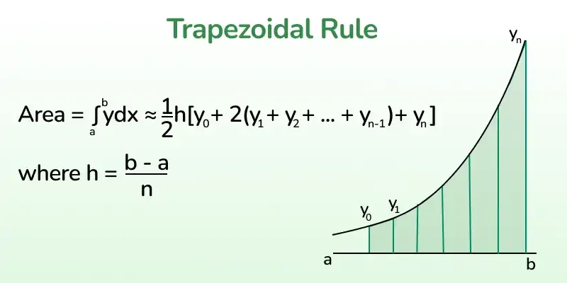
Usually, integrals are computed through summing the heights of a function multiplying them by a certain width, what is called the trapezoidal rule. For high dimensions (multiple integrals) the computation might be difficult, specially when the bounds of the integral are strange or depend on the integration variables.

The ''solution'' to this problem could be training a Neural Network (NN) to do the job for us. Obviously, for 1 variable functions the job could be counterproductive; this is just an exercise to learn TensorFlow.

The example we will use will be the integration through the $(-3,3)$ interval.

📑Preparing the dataset

Firstly, we have to import the libraries that we will use.

import matplotlib.pyplot as plt
import tensorflow as tf
import numpy as np

The dataset to train the model will be a list of polynomial functions (of order 4) and they correspondant area. Since they are polynomial, the area can be calculated analytically (that was the whole starting point).

$$\begin{align} f(x)=&Ax^4+Bx^3+Cx^2+Dx+E \\\ F(x)=&\frac A5x^5 + \frac B4 x^4 + \frac C3 x^3 + \frac D2 x^2 + Ex+K \\\ \int_{-3}^3f(x)dx =& F(3)-F(-3) \end{align}$$

The parameters $A,B,C,D,E,F$ of the function will be randomly generated. So, we make some functions that return all these types of data given a numpy linspace (which is the domain of the function). The type of functions that will be passed to the NN can be found and explored in this desmos project. There, you can check how the functions change when modifying their parameters.

def primitive(A, B, C, D, E, x):
  return A / 5 * x ** 5 + B / 4 * x ** 4 + C / 3 * x ** 3 + D / 2 * x ** 2 + E * x

def integral(Xarray, A, B, C, D, E):
  min = Xarray[0]
  max = Xarray[np.shape(x)[0] - 1]
  return primitive(A, B, C, D, E, max) - primitive(A, B, C, D, E, min)

def polynomial(Xarray):
  A = np.random.uniform(-0.01, 0.01)
  B = np.random.uniform(-0.1, 0.1)
  C = np.random.uniform(-0.1, 0.1)
  D = np.random.uniform(-1, 1)
  E = np.random.uniform(-1, 1)
  dim = np.shape(Xarray)
  return [np.array([[integral(Xarray, A, B, C, D, E)]]), A * Xarray ** 4 + B * Xarray ** 3 + C * Xarray ** 2 + D * Xarray + E]

Now, we prepare $5000$ samples of these functions and slice them into the input and output:

x = np.linspace(-3, 3, 1000)
n_samples = 5000
data = [polynomial(x) for i in range(n_samples)]
input = np.array([data[i][1] for i in range(n_samples)])
output = np.array([data[i][0] for i in range(n_samples)])

We can plot some of them so you get the idea of how the dataset looks:

plt.figure(figsize=(5,5))
for i in range(25):
    plt.subplot(5,5,i+1)
    plt.xticks([])
    plt.yticks([])
    plt.grid(False)
    plt.plot(x, input[i])
    #plt.xlabel(class_names[label])
plt.show()

Finally, we separate the dataset into a training group and a testing one. We will choose $80$% of the data to train our NN and $20$% to test its accuracy.

d_train = input[:int(n_samples * 0.8)]
y_train = output[:int(n_samples * 0.8)]

d_test = input[int(n_samples * 0.8):]
y_test = output[int(n_samples * 0.8):]

Now, everything is ready to train the NN.

🧠Defining and training the Neural Network

The layer scheme of the NN would be clear from a mathematical point of view. If we use a model with 2 layers of this form:

$$\begin{align} \begin{matrix} \begin{pmatrix}x_1\end{pmatrix}\\\ \begin{pmatrix}x_2\end{pmatrix}\\\ \begin{pmatrix}x_3\end{pmatrix}\\\ \vdots\\\ \begin{pmatrix}x_n\end{pmatrix} \end{matrix} \Longrightarrow \begin{pmatrix}I\end{pmatrix} \end{align}$$

Where the final neuron is dense; the NN would eventually learn that the weights ($\omega_i$) are all just the length of the numpy linspace ($\omega=6/1000$) and the bias is $0$. That is,

$$I = \sum_i^nx_i\cdot \omega$$

This formula is the Riemann integral!

So, we don't want to use these type of architecture, since it is too obvious. Instead, we will use a simple 3 layer one:

$$\begin{align} \begin{matrix} \begin{pmatrix}x_1\end{pmatrix}\\\ \begin{pmatrix}x_2\end{pmatrix}\\\ \begin{pmatrix}x_3\end{pmatrix}\\\ \vdots\\\ \begin{pmatrix}x_n\end{pmatrix} \end{matrix} \Longrightarrow \begin{matrix} (\text{hidden})\\\ \begin{pmatrix}y_1\end{pmatrix}\\\ \begin{pmatrix}y_2\end{pmatrix}\\\ \begin{pmatrix}y_3\end{pmatrix}\\\ \vdots\\\ \begin{pmatrix}y_n\end{pmatrix}\\\ \end{matrix} \Longrightarrow \begin{pmatrix}I\end{pmatrix} \end{align}$$

This can be achieved by using a sequence of tf.keras.layers.Dense layers, using as input something with shape x (the input array). The hidden one will have the same shape as the input.

model = tf.keras.Sequential([
    tf.keras.layers.Dense(units=np.shape(x)[0], input_shape=np.shape(x)),
    tf.keras.layers.Dense(units=1)
])

Then, we compile it with the Adam optimizer (using some step parameter that will be figured out by trial-error). The loss function used will be the mean squared error, which is the usual for these cases.

model.compile(loss='mean_squared_error',
              optimizer=tf.keras.optimizers.Adam(0.0001))

To train it, we use the .fit method. We will feed the data in batches of 32 and will relook at the data 20 times (to avoid overfitting), those are called the epochs.

history = model.fit(d_train, y_train, epochs=20, batch_size = 32, verbose=True)

We can plot the loss function in every step (epoch).

plt.xlabel('Epoch Number')
plt.ylabel("Loss Magnitude")
plt.plot(history.history['loss'])
plt.yscale('log')
plt.show()

This is the typical shape of a gradient descent 😎. Now, let's evaluate the accuracy.

🧪Testing

Lucky us, TensorFlow includes a method (.evaluate) to evaluate the NN with some testing data, the d_test,y_test we prepared previously.

test_error = model.evaluate(d_test, y_test, batch_size=32)
print('Mean error:', test_error)

Mean error: 2.9877760421986865e-13

As we can see, the mean error is really low. But, we have to remember that this NN was trained to calculate polynomial areas. So, it is normal that does well at calulating other polynomial areas.

At the end, a NN is an expert recognizing patterns, once you go further, it is expected to fail. So, let's test it with other non-polynomial functions!

The three chosen will be these:

$$\begin{align} f_1(x) =& e^{-x^2}\\\ f_2(x) =& \cos(x)\\\ f_3(x) =& x^2e^{x} \end{align}$$

So, we can test them with the model's predictions using .predict. The areas have been calculated with the desmos project we mentioned before.

def gauss(X):
  return np.exp(-X **2)

def cos(X):
  return np.cos(X)

def fun(X):
  return X ** 3 * np.exp(X)

y2 = np.array([gauss(x)])
predict = model.predict(y2)[0][0]
print("Gaussian")
print("Predicted area:", predict, "\nExpected area:", 1.77241469652)
print("Error:", (1.77241469652 - predict) ** 2, "\n")

y2 = np.array([cos(x)])
predict = model.predict(y2)[0][0]
print("Cosine")
print("Predicted area:", predict, "\nExpected area:", 0.28224001612)
print("Error:", (0.28224001612 - predict) ** 2, "\n")

y2 = np.array([fun(x)])
predict = model.predict(y2)[0][0]
print("Squared and exponential")
print("Predicted area:", predict, "\nExpected area:", 99.5813044537)
print("Error:", (99.5813044537 - predict) ** 2, "\n")

Gaussian
Predicted area: 1.7523017 
Expected area: 1.77241469652
Error: 0.00040453242 


Cosine
Predicted area: 0.30594042 
Expected area: 0.28224001612
Error: 0.00056170975 

Squared and exponential
Predicted area: 241.72617 
Expected area: 99.5813044537
Error: 20205.164 

As it can be seen, it is pretty good at predicting the area of functions which image is the same as the dataset. However, once the function takes large values, the model fails (by far) to predict its area. Again, NN's are experts in recognizing patterns, once they encounter a new case, they fail.

😃Your turn

Now it's your turn to experiment with different functions! You can use the desmos project as a guide to compare theoretical areas to the model's predictions.