- Data Preprocessing
- Feature Scaling
- Standardization
- Normalization
- Encoding Categorical Data
- Mathematical Transformations
- Function Transformation
- Power Transform
- Quantile Transformation
- Encoding Numerical Features
- Discretizationbinning
- Binarization
- Outlier Handling
- Outlier Detection Techniques
- Outlier Handling Techniques
- Handling Missing Values
- Dimension Reduction
- Handling Imbalanced Data
- Metrics
- ML Models
- NLP
-
Formula:
$x' = \frac{x - \text{mean}(x)}{\sigma}$ -
Standardized data has a mean of 0 and a standard deviation of 1.
-
Useful when features are on different scales; works well with algorithms that assume normal distribution.
-
Min-Max Scaling: Scales data to a fixed range, typically [0, 1] or [-1, 1].
-
Formula:
$x' = \frac{x - \text{min}(x)}{\text{max}(x) - \text{min}(x)}$ -
Used for data where negative and positive values are known.
-
-
Max Abs Scaling: Divides each value by the maximum absolute value in the feature, scaling between -1 and 1.
-
Formula:
$x' = \frac{x}{max(|x|)}$ -
Works well with sparse data.
-
-
Robust Scaling: Uses the Interquartile Range (IQR) instead of min and max, making it less sensitive to outliers.
-
Formula:
$x' = \frac{x - \text{median}(x)}{\text{IQR}}$ -
Works well with outliers.
-
-
Ordinal Encoding
Original Feature | Ordinal Feature -----------------|---------------- Poor | 0 Good | 1 Excellent | 2 -
Nominal Encoding (One-Hot Encoding)
Pet Type   | Dog | Cat | Rabbit
-----------|-----|-----|-------
Dog        |  1  |  0  |   0
Cat        |  0  |  1  |   0
Rabbit     |  0  |  0  |   1
- left-skewed data
- right-skewed data
- Formula
-
$x = \frac{x^\lambda - 1}{\lambda}$ for$\lambda \neq 0$ -
$y = \log(x)$ for$\lambda = 0$
-
- Works when the data is strictly positive.
- Formula
$y' = \frac{(y + 1)^\lambda - 1}{\lambda}, \text{ if } \lambda \neq 0, y \geq 0$ $y'= \log(y + 1), \text{ if } \lambda = 0, y \geq 0$ $y'= -\frac{(-y + 1)^{2 - \lambda} - 1}{2 - \lambda}, \text{ if } \lambda \neq 2, y < 0$ $y' = -\log(-y + 1), \text{ if } \lambda = 2, y < 0$
- Works with both positive and negative values.
- based on its cumulative distribution function (CDF)
-
Steps in Quantile Transformation
-
Sort the Data: First, the data is sorted in ascending order
-
Calculate the Rank (or Percentile) for Each Data Point:
$r_i = \frac{i}{n}$ where$i$ is the index of the data point in the sorted list (starting from 1). -
Map the Quantiles to a New Distribution:
-
Uniform Distribution: The simplest form of quantile transformation is to map the ranks directly to a uniform distribution over the range [0, 1]. The transformed value
$y_i$ of$x_i$ is:$y_i = r_i = \frac{i}{n}$ -
Normal Distribution: If you want to transform the data into a normal distribution, you would map the quantiles
$r_i$ to a corresponding value from the inverse cumulative distribution function (CDF) of the standard normal distribution$\Phi^{-1}(r_i)$ .The transformed value
$y_i$ becomes:$y_i = \Phi^{-1}(r_i)$ where$\Phi^{-1}(r_i)$ is the inverse of the normal CDF at the quantile$r_i$ . This maps the data to a normal distribution with mean 0 and variance 1.
-
-
Handling Ties: If there are duplicate values (ties) in the data, the rank
$r_i$ is calculated by averaging the ranks of the tied values. This ensures that the transformed data remains consistent.
-
- Unsupervised Binning: Bins are created without considering target variable labels.
- Uniform Binning (Equal Width)
- Quantile Binning (Equal Frequency)
- K-means Binning
- Supervised Binning: Bin boundaries are created based on information from the target variable.
- Custom Binning: The user defines bins based on domain knowledge or data distribution.
Converts continuous data into binary (0 or 1) values.
-
Binary Encoding Rule:
-
$y_i = 0$ , if$x_i \leq \text{threshold}$ -
$y_i = 1$ , if$x_i > \text{threshold}$
-
-
For Normally Distributed Data (Mean and Standard Deviation Method)
$\text{Lower Bound} = \mu - 3\sigma$ $\text{Upper Bound} = \mu + 3\sigma$ - Any value outside this range is considered an outlier.
-
For Skewed Data (Interquartile Range, IQR Method)
-
Lower Bound:
$Q1 - 1.5 \times \text{IQR}$ -
Upper Bound:
$Q3 + 1.5 \times \text{IQR}$ - Any data point outside this range is considered an outlier.
-
Lower Bound:
-
Percentile Method
- In this method, outliers are identified based on percentiles. Values in the lower or upper extremes (e.g., below the 1st percentile or above the 99th percentile) are marked as outliers.
- This approach is particularly useful when dealing with highly skewed distributions or when specific cutoffs are preferred.
-
Trimming (Removing Outliers)
- Remove the outliers
-
Capping
- Replace the outliers with a set boundary

Remove rows that have missing values but only if
- Check if the missing data is random.
- missing percentage is less than 5%.
- the probability density function (PDF) of numerical columns are similar before and after removal
- the distribution of categorical values are similar before and after removal
| Row | feature1 | feature2 | feature3 |
|---|---|---|---|
| 0 | 1.0 | 2.0 | 1.5 |
| 1 | 2.0 | NaN | 2.5 |
| 2 | NaN | 6.0 | 3.5 |
| 3 | 4.0 | 8.0 | NaN |
| 4 | 5.0 | 10.0 | 5.5 |
We compute the squared Euclidean distance for each pair of rows using only the available (non-missing) values.
| Row 0 | Row 1 | Row 2 | Row 3 | Row 4 | |
|---|---|---|---|---|---|
| Row 0 | 0 | 2 | 20 | 45 | 96 |
| Row 1 | 2 | 0 | 1 | 34.25 | 18 |
| Row 2 | 20 | 1 | 0 | 4 | 20 |
| Row 3 | 45 | 34.25 | 4 | 0 | 5 |
| Row 4 | 96 | 18 | 20 | 5 | 0 |
We modify the squared Euclidean distance to account for missing values using the formula:
where:
- Total Columns = 3 (feature1, feature2, feature3)
- Columns Used = Number of non-missing values used in distance computation.
| Row 0 | Row 1 | Row 2 | Row 3 | Row 4 | |
|---|---|---|---|---|---|
| Row 0 | |||||
| Row 1 | |||||
| Row 2 | |||||
| Row 3 | |||||
| Row 4 |
| Row 0 | Row 1 | Row 2 | Row 3 | Row 4 | |
|---|---|---|---|---|---|
| Row 0 | 0.000 | 1.732 | 5.477 | 9.486 | 16.970 |
| Row 1 | 1.732 | 0.000 | 0.816 | 4.268 | 3.464 |
| Row 2 | 5.477 | 0.816 | 0.000 | 2.000 | 4.472 |
| Row 3 | 9.486 | 4.268 | 2.000 | 0.000 | 2.236 |
| Row 4 | 16.970 | 3.464 | 4.472 | 2.236 | 0.000 |
- Uniform Method: This method uses the average of the feature values of the K nearest neighbors. You can define the number of neighbors (K) and fill in missing values based on their average.
-
Distance Method: In this method, the weighted average of the feature values is calculated, where the weights are the inverse of the non-Euclidean distance:
$\frac{\sum\frac{1}{dist}*\text{feature Value}}{\sum\frac{1}{dist}}$
| Row | feature1 | feature2 | feature3 |
|---|---|---|---|
| 0 | 1.0 | 2.0 | 1.5 |
| 1 | 2.0 | 2.5 | |
| 2 | 6.0 | 3.5 | |
| 3 | 4.0 | 8.0 | |
| 4 | 5.0 | 10.0 | 5.5 |

- Initial Imputation (Fill NaN Values with Mean
- Choose a NaN Value (X) to Impute
- Train a model (e.g., linear regression, decision tree, etc.) where:
- The features (inputs) are a combination of columns b and d (denoted as (b + concat d)).
- The target variable is a combination of the values from columns a and c (denoted as concat a + c).
- After training the model, use the input data from column e (denoted as e) to predict the missing value X.
- Repeat for All Missing Values
- After imputing all missing values in the dataset, update the missing values with the predicted values.
- Instead of filling with the mean, use the newly predicted values as the starting point for the next iteration.
- Repeat this process for several iterations or until the changes in imputed values become minimal between iterations.
- The aim of Principal Component Analysis (PCA) is to find a direction or vector onto which the projection of data points will have the maximum variance. This direction is called the principal component. PCA identifies the directions (principal components) in which the data varies the most and projects the data onto these directions to reduce dimensionality while retaining the most significant information.
-
Mean Centering the Data:
- Subtract the mean of each feature from the dataset, making the data zero-centered (mean-centered).
-
Compute the Covariance Matrix:
-
For an
$n \times m$ matrix$\text{Data}$ , where$n$ is the number of observations (e.g., 1000) and$m$ is the number of features (e.g., 4), calculate the covariance matrix. -
The covariance matrix,
$C$ , is an$m \times m$ (e.g.,$4 \times 4$ ) matrix where each element represents the covariance between two features:$f_1$ $f_2$ $\dots$ $f_m$ $f_1$ $\text{cov}(f_1, f_1)$ $\text{cov}(f_1, f_2)$ $\dots$ $\text{cov}(f_1, f_m)$ $f_2$ $\text{cov}(f_2, f_1)$ $\text{cov}(f_2, f_2)$ $\dots$ $\text{cov}(f_2, f_m)$ $\vdots$ $\vdots$ $\vdots$ $\ddots$ $\vdots$ $f_m$ $\text{cov}(f_m, f_1)$ $\text{cov}(f_m, f_2)$ $\dots$ $\text{cov}(f_m, f_m)$ -
Diagonal elements represent variances, and off-diagonal elements represent covariances between different features.
-
-
Calculate Eigenvalues and Eigenvectors:
-
Solve for the eigenvalues and eigenvectors of the covariance matrix
$C$ . The eigenvalues indicate the amount of variance captured by each principal component. -
The equation for finding eigenvalues
$\lambda$ and eigenvectors$X$ is:$(C - \lambda I)X = 0$ where
$I$ is the identity matrix.
-
-
Select Principal Components:
- Sort the eigenvalues in descending order, and select the top p(e.g., 2) eigenvalues along with their corresponding eigenvectors. These p eigenvectors form a new
$p \times m$ eigenvector matrix (e.g.,$2 \times 4$ ) that will be used for projection.
- Sort the eigenvalues in descending order, and select the top p(e.g., 2) eigenvalues along with their corresponding eigenvectors. These p eigenvectors form a new
-
Project Data onto New Subspace:
-
Transform the original data to a lower-dimensional space by multiplying it with the selected eigenvectors:
$Data_{new} = Data_{MeanCentered} . Eigenvectors$ -
If you reduce from m features to p (e.g., 4 features to 2), the result will be a
$n \times p$ matrix (e.g.,$1000 \times 2$ matrix).
-
Given a dataset with
-
$\mathbf{X} = [\mathbf{x}_1, \mathbf{x}_2, \dots, \mathbf{x}_n]$ represent the dataset with$n$ samples. - Each sample
$\mathbf{x}_i \in \mathbb{R}^d$ is a$d$ -dimensional feature vector. - Let
$\mathbf{X}_j$ be the subset of samples belonging to class$j$ , which has$n_j$ samples.
-
Class Mean Vector:
$m_j = \frac{1}{n_j} \sum_{x \in X_j} x$ -
Within-Class Scatter Matrix: The spread of each class around its own mean.
$S_W = \sum_{j=1}^{c} \sum_{x \in X_j} (x - m_j)(x - m_j)^T$ -
Between-Class Scatter Matrix: How far apart the class means are from the overall mean.
$S_B = \sum_{j=1}^{c} n_j (m_j - m)(m_j - m)^T$ -
Optimization Objective: find a projection vector w that maximizes the ratio of between-class variance to within-class variance.
$J(w) = \frac{w^T S_B w}{w^T S_W w}$ -
Eigenvalue Problem:
$S_B w = \lambda S_W w$ - Compute the eigenvalues and eigenvectors of
$\mathbf{S}_W^{-1} \mathbf{S}_B$ . - Sort the eigenvectors by their corresponding eigenvalues in descending order.
- Select the top
$k$ eigenvectors (where$k \leq c - 1$ ) to form the transformation matrix$\mathbf{W}$ .
- Compute the eigenvalues and eigenvectors of
- Assumptions: LDA assumes that each class follows a Gaussian distribution with identical covariance matrices, and it is sensitive to outliers and class imbalances.
- Aims to maximize the distace b/w classes and minimise the variance within each class' data points
- Computationally Efficient: LDA is faster than some non-linear techniques (e.g., t-SNE or UMAP) because it is a linear method.
- LDA vs. PCA
- PCA: An unsupervised method that focuses on maximizing variance, capturing the most important features regardless of class labels.
- LDA: A supervised method that maximizes class separability, explicitly using class labels to create dimensions that emphasize distinctions between classes.
-
Perform SVD on
$\mathbf{A}$ :- Decompose
$\mathbf{A}$ as:$\mathbf{A} = \mathbf{U} \mathbf{\Sigma} \mathbf{V}^T$ where:-
$\mathbf{U}$ is an$m \times m$ matrix of the left singular vectors. -
$\mathbf{\Sigma}$ is an$m \times n$ diagonal matrix containing the singular values in descending order. -
$\mathbf{V}^T$ is the transpose of an$n \times n$ matrix$\mathbf{V}$ , which contains the right singular vectors.
-
- Decompose
-
Truncate
$\mathbf{U}$ ,$\mathbf{\Sigma}$ , and$\mathbf{V}^T$ :- Since the goal is to reduce
$\mathbf{A}$ to an$m \times 2$ matrix, we keep only the top 2 singular values and the corresponding left and right singular vectors. - Define:
-
$\mathbf{U}_2$ : the first 2 columns of$\mathbf{U}$ , with dimensions$m \times 2$ . -
$\mathbf{\Sigma}_2$ : a$2 \times 2$ diagonal matrix containing the top 2 singular values. -
$\mathbf{V}_2^T$ : the first 2 rows of$\mathbf{V}^T$ , with dimensions$2 \times n$ .
-
Then, we can approximate
$\mathbf{A}$ as:$\mathbf{A} \approx \mathbf{U}_2 \mathbf{\Sigma}_2 \mathbf{V}_2^T$ - Since the goal is to reduce
-
Compute the Reduced Representation
$\mathbf{A}'$ :- To get the reduced matrix
$\mathbf{A}'$ of dimensions$m \times 2$ , multiply$\mathbf{U}_2$ and$\mathbf{\Sigma}_2$ :$\mathbf{A}' = \mathbf{U}_2 \mathbf{\Sigma}_2$ This yields an$m \times 2$ matrix$\mathbf{A}'$ , which is the desired reduced representation.
- To get the reduced matrix
The following steps outline the SVD calculation in detail, which are foundational for deriving
-
Calculate Eigenvalues and Eigenvectors of
$A \cdot A^T$ :- Compute
$A \cdot A^T$ . - Find the eigenvalues and eigenvectors of
$A \cdot A^T$ . - These eigenvectors form the columns of
$\mathbf{U}$ .
- Compute
-
Normalize Each Eigenvector:
- Normalize each eigenvector of
$A \cdot A^T$ to ensure the columns of$\mathbf{U}$ have unit length.
- Normalize each eigenvector of
-
Stack Eigenvectors of
$A \cdot A^T$ Based on Eigenvalues (Descending):- Sort the eigenvalues in descending order.
- Stack the corresponding normalized eigenvectors horizontally to form
$\mathbf{U}$ .
-
Calculate Eigenvalues and Eigenvectors of
$A^T \cdot A$ :- Compute
$A^T \cdot A$ . - Find the eigenvalues and eigenvectors of
$A^T \cdot A$ . - These eigenvectors form the columns of
$\mathbf{V}$ .
- Compute
-
Normalize Each Eigenvector:
- Normalize each eigenvector of
$A^T \cdot A$ so the columns of$\mathbf{V}$ have unit length.
- Normalize each eigenvector of
-
Stack Eigenvectors of
$A^T \cdot A$ Based on Eigenvalues (Descending):- Sort the eigenvalues in descending order.
- Stack the corresponding normalized eigenvectors horizontally to form
$\mathbf{V}$ .
-
Transpose
$V$ :- Compute
$V^T$ , which is used in the SVD decomposition.
- Compute
-
Form
$\Sigma$ :- Use a zero matrix of dimensions
$m \times n$ . - Populate this matrix with the square roots of the eigenvalues of
$A^T \cdot A$ along the diagonal, in descending order. These values are the singular values of$A$ .
- Use a zero matrix of dimensions
This process yields the matrices

-
Train a k-NN model on minority class observations:
- Identify the k nearest neighbors for each minority class sample (commonly ( k = 5 )).
-
Create synthetic data:
- Select 1 example randomly from the minority class.
-
Select one neighbor randomly from its
$k$ -nearest neighbors. - Extract a random number
$\alpha$ between 0 and 1 for interpolation. - Generate the synthetic sample using the formula:
$\text{Synthetic sample} = \text{Original sample} + \alpha \times (\text{Neighbor} - \text{Original sample})$
- Repeat the process to create multiple synthetic samples.
- Combine the original dataset with synthetic samples to form a balanced dataset.

| Metric | Formula | Description |
|---|---|---|
| Accuracy | Greater values indicate better performance. | |
| Precision | Greater values indicate better performance. | |
| Recall | Greater values indicate better performance. | |
| F1-score | Greater values indicate better performance. | |
| Log Loss | Lower values indicate better performance. |
| Metric | Formula | Description |
|---|---|---|
| Mean Absolute Error (MAE) | ||
| Mean Squared Error (MSE) | ||
| Root Mean Squared Error (RMSE) | ||
| R-squared (R²) | Greater values indicate better performance. | |
| Adjusted R-squared |
useful for comparing models with different feature sets. |
-
$X$ : The matrix of input features (with dimensions$1000 \times 10$ , where$1000$ is the number of observations and$9$ is the number of predictors and first column containing 1 only). -
$Y$ : The vector of observed outcomes (with dimensions$1000 \times 1$ ). -
$\beta$ : The vector of estimated coefficients (with dimensions$10 \times 1$ ). -
$\hat{Y}$ : The vector of predicted values (with dimensions$1000 \times 1$ ).
Predicting Values (
1. Closed Form Formula / The Ordinary Least Squares (OLS)
2. Non-Closed Form Formula Run these for n epoches
Suppose we have three features and we want apply degree 2 polynonial features then calculate or make ney features ->
- Here
$I = I$ where$I[0][0] = 0$ - Example
0 0 0 0 1 0 0 0 1
- Example
-
As
$\lambda$ increases, value only decreases but never goes to 0
-
For
$m > 0$ $m = \frac{\sum (y_i - \bar{y})(x_i - \bar{x}) - \lambda}{\sum (x_i - \bar{x})^2}$ -
For
$m = 0$ $m = \frac{\sum (y_i - \bar{y})(x_i - \bar{x})}{\sum (x_i - \bar{x})^2} $ -
For
$m < 0$ $m = \frac{\sum (y_i - \bar{y})(x_i - \bar{x}) + \lambda}{\sum (x_i - \bar{x})^2}$ -
Lasso regression is used for feature selection, for greater values of
$\lambda$ .
-
How coefficients get affected as
$\lambda$ increases- For Ridge →
$m \approx 0$ but$m \neq 0$ - For Lasso →
$m = 0$
- For Ridge →
-
More the value of
$m$ the higher & more it decreases fully as$\lambda$ increases..png)
-
Bias-Variance tradeoff
.png)

-
Impact on loss function
- As
$\lambda$ increases, minimum loss increases. - As
$\lambda$ increases,$m$ gets close to 0..png)
- As
.png)
Loss, L = ∑i=1 (̂yi - yi)2 + α ∑i=1 |wi| + β ∑i=1 wi2
- Use when we do not know if we have to apply Ridge or Lasso regression.
- Ridge → when every independent variable has some importance.
- Lasso → when we want to train the model on a subset of variables instead of all variables.
- If a point is in wrong region then move line towards the point
- Do not work bcoz it stops once a boundry is created thus not give best result
- ALGORITHM
- for n in range(1000):
- select a random col i
$W_{new} = W_{old} + \eta(Y_i - \hat{Y}_i)x_i^T$
$\hat{Y} = X W$
- select a random col i
-
$W$ : The updated weight vector of dimension 10×1. -
$\eta$ : The learning rate. -
$x_i$ : The feature vector corresponding to the$i$ th data point of dimension 1×10.
- for n in range(1000):

- Here we use sigmoid function
- ALGORITHM
- for n in range(1000):
- select a random col i
$W_{new} = W_{old} + \eta(Y_i - \hat{Y}_i)x_i^T$
$\hat{Y} = \sigma(X W)$
- select a random col i
- for n in range(1000):
- ALGORITHM
- For epoch in range(10):
$W = W_{n-1} + \frac{\eta}{m} X^T (Y - \hat{Y})$ $\hat{Y} = \sigma(X W)$
- For epoch in range(10):
1. Method-One
- Apply one hot encoding

- Train model for each column
2. Method-Two
- We can apply L1, L2, elatic net regression
It based on the concept "You are the average of the five people you spend the most time with"
- Normalize the Data
- Find the Distance of All Points:
- Use Euclidean distance
- Identify the K Nearest Neighbors
- Determine the Output:
- KNN for Classification:
- Majority Vote: The label of the query point is determined by the majority class among the K nearest neighbors.
- KNN for Regression:
- Average (or Weighted Average): The predicted value for the query point is the average (or a weighted average) of the values of the K nearest neighbors.
- KNN for Classification:
| Toss | Venue | Outlook | Result |
|---|---|---|---|
| Won | Mumbai | Overcast | Won |
| Lost | Chennai | Sunny | Won |
| Won | Kolkata | Sunny | Won |
| Won | Chennai | Sunny | Won |
| Lost | Mumbai | Sunny | Lost |
| Won | Mumbai | Sunny | Lost |
| Lost | Chennai | Overcast | Lost |
| Won | Kolkata | Overcast | Lost |
| Won | Mumbai | Sunny | Won |
For numerical features, the Naive Bayes classifier uses the Gaussian (normal) distribution:
You would apply this formula to compute the probability density for numerical values in each class, such as "Won" or "Loss" by finding the std and mean for that class and putting those and value of x in the formula to get probablity.
Pseudo code
- Begin with your training dataset, which should have some feature variables and classification or regression output.
- Determine the “best feature” in the dataset to split the data on
- Split the data into subsets that contain the correct values for this best feature. This splitting basically defines a node on the tree i.e each node is a splitting point based on a certain feature from our data.
- Recursively generate new tree nodes by using the subset of data created from step 3.
Advantages
- The cost of using the tree for inference is logarithmic in the number of data points used to train the tree
Disadvantages
- Overfitting
- Prone to errors for imbalanced datasets
where
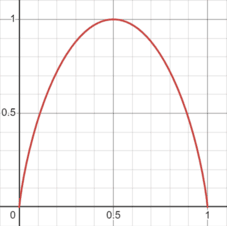
Observation
- For a 2 class problem the min entropy is 0 and the max is 1
- For more than 2 classes the min entropy is 0 but the max can be greater than 1
- Both
$log_2$ or$log_e$ can be used to calculate entropy
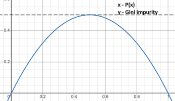
Some times Gini Impurity may give balanced tree incomparision to entropy
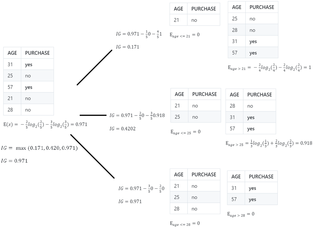
- Calculate Entropy / Gini impurity of Parent
- Calculate Information Gain for all the columns
- Calculate Entropy / Gini impurity for Children
- Calculate weighted Entropy / Gini impurity of Children
- Whichever column has the highest Information Gain(maximum decrease in entropy) the algorithm will select that column to split the data.
- Once a leaf node is reached ( Entropy = 0 ), no more splitting is done.
- Sort the data on the basis of numerical column
- Split the entire data on the basis of every value of numerical column
- Calculate Information Gain for each split
- Select Max Information Gain and it is the Information Gain for that column
- Calculate Standard Deviation of the Parent Node
- Calculate Information Gain for all the columns
- Calculate Standard Deviation for Child Nodes
- For Categorical Features: Split the data into different groups based on the unique labels of the categorical feature. Compute the standard deviation of the target variable for each group (child node).
- For Numerical Features: Perform repeated splits for each unique value of the numerical feature. For each possible split, divide the data into two groups (child nodes) and calculate the standard deviation of the target variable within each group.
- Calculate Weighted Standard Deviation of Children
- Calculate Information Gain: Information Gain = Std of Parent − Weighted Std of Children
- Calculate Standard Deviation for Child Nodes
- Whichever column has the highest Information Gain the algorithm will select that column to split the data.
- The algorithm recursively repeats the process for each child node until a stopping criterion is met.
- At each leaf node, the output is the mean of the target variable values within that node..
Calculate this for each node t and which has split for feature
-
$Feature Importance(i)$ : Importance score for feature$i$ . -
$N_t$ : Number of samples at node$t$ . -
$N$ : Total number of samples. -
$\text{impurity}$ : Impurity measure at node$t$ (e.g., Gini impurity, entropy). -
$N_{t_r}$ : Number of samples in the right child node after the split. -
$N_{t_l}$ : Number of samples in the left child node after the split. -
$\text{Right Impurity}$ : Impurity of the right child node of node t. -
$\text{Left Impurity}$ : Impurity of the left child node of node t.
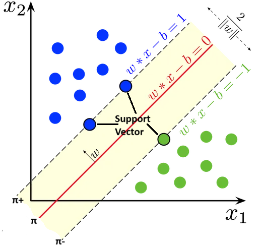
- The aim of this is to
- maximise the distance between
$π_+$ and$π_-$ - minimise the distance distance of wrong output points to there repective correct margin plane
- maximise the distance between
Below objective function seeks to minimize a combination of the margin (through the regularization term) and the misclassification error (through the slack variables). The goal is to find the optimal
$\arg\min_{w*, b*} \left( Margin Error + Classification Error\right)$ $\arg\min_{w*, b*} \left( \frac{1}{2} ||w||^2 + C \sum_{i=1}^n \zeta_i \right)$
where:
We use Kernels for non linear seperable data
Based on the concept of the wisdom of the crowd, decisions made by multiple models have a higher chance of being correct. Ensemble learning helps convert a low-bias, high-variance model into a low-bias, low-variance model because the random/outliers are distributed among various models instead of going to a single model.
-
Voting Ensemble: In this approach, different models of various types, such as SVM, Decision Tree, and Logistic Regression, calculate results. For classification tasks, the output with the highest frequency is selected as the final result, or we add probabilities of each class obtained from models. For regression tasks, the mean of the outputs is calculated.
-
Stacking: In stacking, different models of various types, such as SVM, Decision Tree, and Logistic Regression, are used to calculate results. The outputs of these models are then used to train a final model, such as KNN, to obtain the final output. This final model effectively assigns a weight to each previous model's prediction.
-
Bagging: In bagging, multiple models of the same type (i.e., using the same algorithm) are trained. Each model is trained on a different sample of the data, not the entire dataset. The final result is determined by averaging (for regression) or using majority voting (for classification).
-
Boosting: In boosting, different models are connected in series. The error made by one model is passed on to the next model in the series, which attempts to correct it. This process continues, with each subsequent model focusing on the errors of the previous one.
We are given 3 models, each having an accuracy of 0.7.
                                    1
                                  /   \
                                /       \
                              /           \
                            /               \
                          /                   \
                        0.7                   0.3
                        / \                   / \
                      /     \               /     \
                    /        \             /       \
                   0.7       0.3        0.7         0.3
                  / \        / \        / \         / \
               0.7   0.7   0.7  0.3   0.7  0.3    0.7  0.3
                ✔    ✔     ✔         ✔
Final Accuracy:
- Hard Voting: The output with the highest frequency is selected as the final result, i.e., argmax().
- Soft Voting: We add probabilities of each class obtained from models and then select the class with the highest value.

- Split the training data into two parts.
- Train base models on the first part.
- Use the second part to generate predictions using stacked models, which are used as input for the meta-model.
- The meta-model is trained on these predictions.
- Split the training data into K folds.
- Train K models of the same type, each leaving out one fold for predictions.
- Predictions from the out-of-fold data are used to train the meta-model.
- The meta-model is trained on the stacked predictions.
- Finally, the base models are retrained on the entire dataset.

-
Row Sampling with Replacement: Standard bagging technique where data is sampled with replacement.
-
Pasting: Row sampling without replacement.
-
Random Subspaces: Column sampling, which can be done with or without replacement.
-
Random Patches: Both row and column sampling are performed, with or without replacement.
Out-of-Bag (OOB) Error: Approximately 37% of samples are not used for model training, so this data can be used for testing the model.
-
Initial Weights: For a dataset with
$n$ samples, initialize the weight for each row/sample as$\frac{1}{n}$ .$w_i = \frac{1}{n}, \quad \text{for all } i \text{ where } i \text{ is the row number}$
x y $w_i$ $\frac{1}{n}$ -
Train a Weak Learner: Train a decision tree of depth 1 (also known as a decision stump) using the current weights.
-
Predictions: Use the trained decision stump to make predictions on the training data.
x y $w_i$ $\hat{y}$ $\frac{1}{n}$ -
Error Calculation: Calculate the error
$\epsilon$ of the stump, which is the sum of the weights of the misclassified samples:-
$\epsilon = w_i \cdot I$ . Here,$I : (\hat{y}_i != y_i)$ is the indicator function that returns 1 if the prediction is incorrect and 0 if correct.
x y $w_i$ $\hat{y}$ $\epsilon$ $\frac{1}{n}$ -
-
Performance of Stump
$\alpha$ : Calculate the performance of the stump (also called the weight of the weak learner):$\alpha = \frac{1}{2} \log \left(\frac{1 - \sum \epsilon}{\sum \epsilon}\right)$
-
Update Weights: Update the weights of the samples based on their prediction outcome:
- If the prediction is correct:
$w_i^{\text{new}} = w_i \cdot e^{-\alpha}$ - If the prediction is incorrect:
$w_i^{\text{new}} = w_i \cdot e^{\alpha}$
x y $w_i$ $\hat{y}$ $\epsilon$ $w_i^{\text{new}}$ $\frac{1}{n}$ - If the prediction is correct:
-
Normalize Weights: Normalize the updated weights so that they sum to 1:
$w_i^{\text{new normal}} = \frac{w_i^{\text{new}}}{\sum_{j=1}^n w_j^{\text{new}}}$ x y $w_i$ $\hat{y}$ $\epsilon$ $w_i^{\text{new}}$ $w_i^{\text{new normal}}$ $\frac{1}{n}$ -
Make Bins: Create bins corresponding to the normalized weights. The bins are cumulative sums of the weights, which will be used to sample the data points for the next iteration.
| x | y | ||||||
|---|---|---|---|---|---|---|---|
-
Generate Random Numbers: Generate random numbers between 0 and 1. Each random number corresponds to a bin, and the row whose bin it falls into is selected for training the next weak learner.
-
This process is repeated for a specified number of iterations or until a desired accuracy is achieved and for iteration make sure to use to use
$w_i = \frac{1}{n}$ . -
The final model is a weighted sum of all the weak learners.
$H(x) = \text{sign} \left( \sum_{n=1}^{N} \alpha_n \cdot h_n(x) \right)$
- ALGORITHM:
prediction = mean(y)  # Initial prediction, starting with the mean of the target values
models_list.append(Mean_Model)  # Store the initial model

for i in range(1, n_estimators):  # Loop to build subsequent models
    residual = y - prediction  # Compute residuals
    tree = tree.fit(X, residual)  # Train a new model on residuals
    models_list.append(tree)  # Add the trained model to the list
    prediction += η * tree.predict(X)  # Update the prediction with scaled predictions from the new model

result = models_list[0](X) + models_list[1](X) + models_list[2](X)M_0(X) + ...
-
Initialize Log Odds:
-
Compute the initial log odds:
$\text{log odds} = \ln\left(\frac{\text{Count of Ones}}{\text{Count of Zeros}}\right)$ -
Append the initial log odds to the
models_listas the first model:modelsList.append(log_odds)
-
-
Loop Over Each Estimator:
- For each
$i$ from 1 to$n_{\text{estimators}}$ :-
Calculate the initial probability:
$\text{prob} = \frac{1}{1 + e^{-\text{log odds}}}$ -
Calculate residuals for the current predictions:
$\text{residual} = y - \text{prob}$ -
Train a weak learner on residuals:
WeakLearner = tree.fit(X, residual)
-
Identify the leaf node number for each data point in the tree.
-
For each leaf node, compute log loss:
$\text{log loss} = \frac{\sum \text{Residual}}{\sum[\text{PrevProb} \times (1 - \text{PrevProb})]}$ -
Append the trained model (with calculated log losses in the leaf nodes) to
models_list: modelsList.append(tree) -
For each point, update
log_lossby adding the weighted log loss from the new tree:$\text{log loss} += \eta \cdot (\text{log loss from tree})$
-
- For each
-
Calculate Final Log Loss Prediction:
- Aggregate the log losses from each model in
models_list:$\text{log loss} = modelsList [0] (X) + \eta \cdot modelsList [1] (X) + \eta \cdot modelsList [2] (X) + \dots$
- Aggregate the log losses from each model in
-
Convert Log Loss to Final Probability:
$\text{prob} = \frac{1}{1 + e^{-\text{log odds}}}$
Given:
- A dataset
$\left( (x_i, y_i) \right)_{i=1}^n$ . - A differentiable loss function
$L(y, F(x))$ where$L(y, F(x)) = \frac{1}{2} (y - F(x))^2$ , which is the squared error loss. - A maximum number of boosting iterations
$M$ .
The goal is to build an additive model
-
Initialize the Base Model:
-
Start by initializing the model
$f_0(x)$ as the constant that minimizes the loss. For squared error loss, this is the mean of$y$ :$$f_0(x) = \arg \min_{\gamma} \sum_{i=1}^N L(y_i, \gamma) = \text{Mean}(y)$$
-
-
Boosting Loop:
-
For
$m = 1$ to$M$ :a. Compute Residuals:
-
For each data point
$i$ , compute the residual$r_{im}$ , which represents the negative gradient of the loss function with respect to$f(x_i)$ evaluated at$f_{m-1}(x)$ :$r_{im} = -\left( \frac{\partial L(y_i, f(x_i))}{\partial f(x_i)} \right)_{f=f(m-1)} $ $r_{im} = y_i - f_{m-1}(x_i)$ -
This residual measures the error between the actual
$y_i$ and the model prediction$f_{m-1}(x_i)$ .
b. Fit a Regression Tree:
- Fit a regression tree to the targets
$r_{im}$ , producing terminal regions$R_{jm}$ for$j = 1, 2, \ldots, J_m$ , where$J_m$ is the number of terminal nodes (leaves) in the tree.
c. Compute Terminal Node Predictions:
-
For each region
$R_{jm}$ , compute the optimal value$\gamma_{jm}$ that minimizes the loss over the points in$R_{jm}$ . Since the loss function is squared error, this$\gamma_{jm}$ is the average residual for points in$R_{jm}$ :$$\gamma_{jm} = \arg \min_{\gamma} \sum_{x_i \in R_{jm}} L(y_i, f_{m-1}(x_i) + \gamma)$$ -
For squared error loss,
$\gamma_{jm}$ is the mean of$r_{im}$ for$x_i \in R_{jm}$ .
d. Update the Model:
-
Update
$f_m(x)$ by adding the scaled contributions of the fitted tree:$f_m(x) = f_{m-1}(x) + \eta \sum_{j=1}^{J_m} \gamma_{jm} 1(x \in R_{jm})$ -
Here,
$\eta$ is a learning rate that controls the contribution of each tree.
-
-
-
Final Output:
- After
$M$ iterations, output the final model$f_M(x)$ , which is the sum of the initial model and the contributions from all$M$ boosting steps.
- After
- Flexiblity
- Cross Platform - For windows, Linux
- Multiple Language Support - Multiple Programing Lang
- Integration with other libraries and tools
- Support all kinds of ML problems - Regression, classification, Time Series, Ranking
- Speed - Almost 1/10th time of normal time taken by other ML algos
- Parallel Processing - Apply parallel processing in creation of decision tree, n_jobs = -1
- Optimized Data Structures - Store data in column instead of rows
- Cache Awareness
- Out of Core computing - tree_method = hist
- Distributed Computing
- GPU Support - tree_method = gpu_hist
- Performance
- Regularized Learning Objective
- Handling Missing values
- sparsity Aware Spit Finding
- Efficient Spit Finding(Weighted Quantile Sketch + Approximate Tree Learning) - Instead of spliting on each point in a column we can divide the data in bins
- Tree Pruning
-
Initialize with the Mean Model:
- Set the initial prediction for all data points as the mean of the target variable,
$\text{prediction} = \text{mean}(y)$ . - Store this initial mean model in
models_list.
- Set the initial prediction for all data points as the mean of the target variable,
-
Iterative Training with Trees:
- For each iteration
$i$ from 1 ton_estimators:-
Calculate Residuals:
$\text{residual} = y - \text{prediction}$ -
Build a Decision Tree:
- Train a decision tree based on a custom "Similarity Score," defined as:
$\text{Similarity Score} = \frac{\left(\sum \text{ residuals}\right)^2}{\text{Count of residuals} + \lambda}$ - For each split in the tree:
- Calculate Similarity Score for the tree nodes.
- Determine splits based on the criterion where
$Gani$ is maximized:$Gani = SS_{\text{right}} + SS_{\text{left}} - SS_{\text{parent}}$ - Select the split that maximizes
$Gani$ .
- Set the output at a node:
$\frac{\sum \text{ Residuals}}{\text{Count of residuals} + \lambda}$
- Train a decision tree based on a custom "Similarity Score," defined as:
-
Update Prediction:
- Add the tree's prediction, scaled by a learning rate
$\eta$ , to the cumulative prediction:$\text{prediction} += \eta \times \text{tree.predict}(X)$
- Add the tree's prediction, scaled by a learning rate
-
Calculate Residuals:
- For each iteration
-
Final Prediction Aggregation:
- Combine predictions from all models (starting with the mean model) in
models_list:$\text{result} =$ models_list[0](X) +$\eta.$ models_list[0](X) +$\eta.$ models_list[0](X) +$\dots$
- Combine predictions from all models (starting with the mean model) in
-
Initialize Log Odds:
- Compute the initial log odds:
$\text{log odds} = \ln\left(\frac{\text{Count of Ones}}{\text{Count of Zeros}}\right)$ - Append the initial log odds to the
models_listas the first model: modelsList.append(log_odds)
- Compute the initial log odds:
-
Loop Over Each Estimator:
- For each
$i$ from 1 to$n_{\text{estimators}}$ :- Calculate the initial probability:
$\text{prob} = \frac{1}{1 + e^{-\text{log odds}}}$ - Calculate residuals for the current predictions:
$\text{residual} = y - \text{prob}$ -
Build a Decision Tree:
- Train a decision tree based on a custom "Similarity Score," defined as:
$\text{Similarity Score} = \frac{\left(\sum \text{ residuals}\right)^2}{\sum[\text{PrevProb}×(1-\text{PrevProb})] + \lambda}$ - For each split in the tree:
- Calculate Similarity Score for the tree nodes.
- Determine splits based on the criterion where
$Gani$ is maximized:$Gani = SS_{\text{right}} + SS_{\text{left}} - SS_{\text{parent}}$ - Select the split that maximizes
$Gani$ .
- Set the output at a node:
$\text{log loss} = \frac{\sum \text{Residual}}{\sum[\text{PrevProb} \times (1 - \text{PrevProb})] + \lambda}$
- Train a decision tree based on a custom "Similarity Score," defined as:
- Append the trained model to
models_list: modelsList.append(tree) - For each point, update
log_lossby adding the weighted log loss from the new tree:$\text{log loss} += \eta \cdot (\text{log loss from tree})$
- Calculate the initial probability:
- For each
-
Calculate Final Log Loss Prediction:
$\text{Total log loss} = modelsList [0] (X) + \eta \cdot modelsList [1] (X) + \eta \cdot modelsList [2] (X) + \dots$ -
Convert Log Loss to Final Probability:
$\text{prob} = \frac{1}{1 + e^{-\text{log odds}}}$
- The loss term measures how well the predictions match the target values.
- The regularization term
$\Omega$ controls the complexity of the newly added model$f_t(x_i)$ , often defined as:$\Omega(f) = \gamma T + \frac{1}{2} \lambda |w|^2,$ where$T$ is the number of leaves,$w$ are the leaf weights, and$\gamma, \lambda$ are regularization hyperparameters.
for a tree Node
for regression:
| Bagging | Random Forest |
|---|---|
| In Bagging, feature sampling (or selection) is done before training each decision tree. A subset of features is chosen, and the entire tree uses only this subset of features to make splits. | In Random Forest, feature sampling occurs at each split in the tree. A random subset of features is chosen at each node, and the feature with the best Information Gain or Gini Index is used to make the split. |
| This approach introduces less randomness to individual trees, as the same set of features is used throughout each tree. This can lead to lower variance if the features chosen are highly relevant. | By selecting a different subset of features at each split, Random Forest increases the diversity of the trees, helping to reduce overfitting and increasing model robustness by creating a more diverse "forest" of trees. |
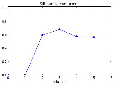
For each cluster, calculate the squared distance of other points in the same cluster to the centroid and sum them. Calculate for each cluster.
Calculate the number of clusters for which increasing the number of clusters does not decrease WCSS.
The silhouette coefficient
Where:
-
$S(i)$ is the silhouette coefficient for data point$i$ . -
$a(i)$ is the average distance between$i$ and all the other data points in the same cluster as$i$ . -
$b(i)$ is the smallest average distance from$i$ to all clusters to which$i$ does not belong. In other words, it's the distance to the nearest cluster that$i$ is not a part of.
The silhouette coefficient
-
$S(i)$ close to 1 indicates that the data point is well-clustered. -
$S(i)$ close to 0 indicates that the data point is on or very close to the decision boundary between two neighboring clusters. -
$S(i)$ close to -1 indicates that the data point might have been assigned to the wrong cluster.
Find the average
Choose the cluster where
Where:
-
$\text{CH}$ is the Calinski-Harabasz Score. -
$\text{Tr}(B_k)$ is the trace of the between-cluster dispersion matrix. -
$\text{Tr}(W_k)$ is the trace of the within-cluster dispersion matrix. -
$n$ is the total number of data points. -
$k$ is the number of clusters.
This measures the dispersion between different clusters. It is defined as:
Where:
-
$n_j$ is the number of data points in cluster$j$ . -
$\mu_j$ is the centroid of cluster$j$ . -
$\mu$ is the overall mean of the data.
This measures the dispersion within each cluster. It is defined as:
Where:
-
$x_i$ are the data points in cluster$C_j$ . -
$\mu_j$ is the centroid of cluster$j$ .
Higher Score: Indicates that clusters are well-separated and compact.
Lower Score: Suggests overlapping or poorly defined clusters.
- Epsilon (ε): This parameter defines the radius of the neighborhood around a point. It is the maximum distance between two points for one to be considered as in the neighborhood of the other.
- MinPoints: This is the minimum number of points required to form a dense region (including the point itself).
- Core Points:
- A Core Point is a point that has at least
MinPoints(including itself) within its ε-radius neighborhood.
- A Core Point is a point that has at least
- Boundary Points:
- A Boundary Point is a point that has fewer than
MinPointswithin its ε-radius neighborhood but is has atleast one core Point in the ε-radius.
- A Boundary Point is a point that has fewer than
- Noise Points:
- Noise Points, also known as outliers, are points that are neither Core Points nor Boundary Points.
Density-connected means that
- Identify all points as either core point, border point or noise point
- For all of the unclustered core points
- Create a new cluster
- add all the points that are unclustered and density connected to the current point into this cluster
- For each unclustered border point assign it to the cluster of nearest core point
- Leave all the noise points as it is.
- Calculate distances between each pair of data points (e.g., using Euclidean distance) and store them in a matrix.
- Treat each data point as its own cluster.
- Repeat the following steps until only one cluster remains:
- a. Merge the Two Closest Clusters: Identify and merge the pair of clusters with the smallest distance.
- b. Update the Proximity Matrix: Recalculate distances between the newly formed cluster and the remaining clusters based on the chosen linkage criteria (e.g., minimum, maximum, average).
- Continue until all data points are merged into a single cluster, resulting in a hierarchy of clusters.
- Single Linkage (Minimum Linkage)
- Definition: Distance between two clusters is the minimum distance between any point in one cluster and any point in the other.
- Characteristics:
- Tends to create elongated, chain-like clusters.
- Disadvantage: Highly sensitive to noise or outliers.
- Complete Linkage (Maximum Linkage)
- Definition: Distance between two clusters is the maximum distance between any point in one cluster and any point in the other.
- Characteristics:
- Tends to form compact, spherical clusters.
- Disadvantage: May break large clusters into smaller sub-clusters.
- Average Linkage
- Definition: Distance between two clusters is the average distance between all pairs of points, with one point from each cluster.
- Characteristics:
- Balances the traits of single and complete linkage.
- Less sensitive to outliers compared to single linkage.
- Ward's Method
- Definition: Measures the increase in variance when clusters are merged by calculating the difference in squared distance sums before and after merging clusters.
- Characteristics:
- Creates compact, spherical clusters.
- Minimizes within-cluster variance at each step.
-
Plot the Dendrogram
-
Cut the Dendrogram Horizontally
- Visually inspect the dendrogram and make a horizontal cut at a certain height to define the number of clusters.
-
Find the Longest Vertical Line
- Identify the longest vertical line that does not intersect with any other line, indicating the biggest distance between merged clusters and a natural division.
-
Determine the Number of Clusters
- The ideal number of clusters corresponds to the number of clusters below the horizontal cut through the longest vertical line.
- Lowercasing
Convert all text to lowercase for uniformity. - Remove HTML Tags
Eliminate HTML tags like<div>or<p>to retain only the plain text. - Remove URLs
Strip out any web links from the text. - Remove Punctuation
Remove punctuation marks to simplify the text. - Chat Word Treatment
Replace common chat abbreviations or slang (e.g., 'u' → 'you', 'r' → 'are'). - Spelling Correction
Correct misspelled words to their standard forms. - Removing Stop Words
Exclude common words like "and", "is", and "the" that do not contribute much meaning. - Handling Emojis
Remove or replace emojis with their textual description. - Tokenization
- Word Tokenization: Break the text into individual words.
- Sentence Tokenization: Divide the text into sentences.
- Stemming
Reduce words to their root forms, even if the resulting word lacks meaning (e.g., "running" → "run"). - Lemmatization
Reduce words to their meaningful base forms (e.g., "better" → "good").
- Corpus: A collection of text data used for analysis or training models.
- Vocabulary: The unique set of words or tokens in the corpus.
- Document: A single piece of text (e.g., a sentence, paragraph, or article) in the corpus.
- Word: An individual token from the vocabulary.
-
Steps:
- Identify the Vocabulary from the corpus.
- Represent each word using a sparse vector based on the vocabulary, with a single "1" indicating the word's presence.
-
Example:
Document Content D1 people watch campusx D2 campusx watch campusx D3 people write comment D4 campusx write comment Vocabulary = [people, watch, campusx, write, comment]
Document Content Vector D1 people watch campusx [ [1,0,0,0,0], [0,1,0,0,0], [0,0,1,0,0] ] D2 campusx watch campusx [ [0,0,1,0,0], [0,1,0,0,0], [0,0,1,0,0] ] D3 people write comment [ [1,0,0,0,0], [0,0,0,1,0], [0,0,0,0,1] ] D4 campusx write comment [ [0,0,1,0,0], [0,0,0,1,0], [0,0,0,0,1] ] -
Pocs:
- Intutive
- Easy Implementation
-
Cons:
- Sparsity
- No Fixed Size
- Out Of Vocabulary
- No campturing of semantic
-
Steps:
- Identify the Vocabulary.
- Represent each document as a fixed-size vector where each unit is the count of a word in the document.
-
Example:
Document Content D1 people watch campusx D2 campusx watch campusx D3 people write comment D4 campusx write comment Vocabulary = [people, watch, campusx, write, comment]
Document Content Vector Binary Vector D1 people watch campusx [1,1,1,0,0] [1,1,1,0,0] D2 campusx watch campusx [0,1,2,0,0] [0,1,1,0,0] D3 people write comment [1,0,0,1,1] [1,0,0,1,1] D4 campusx write comment [0,0,1,1,1] [0,0,1,1,1] -
Pocs:
- Intutive
- Easy Implementation
- Fixed Size
-
Cons:
- Sparsity
- Out Of Vocabulary
- Ordering Get Changed
- No campturing of semantic
-
Steps:
- Build a vocabulary using N-word combinations.
- Represent each document as a vector where each unit indicates the count of N-grams.
-
Example:
Document Content D1 people watch campusx D2 campusx watch campusx D3 people write comment D4 campusx write comment Vocabulary = [people watch, watch campusx, campusx watch, watch campusx, people write, write comment, campusx write]
Document Content Vector D1 people watch campusx [1, 1, 0, 0, 0, 0, 0] D2 campusx watch campusx [0, 0, 1, 1, 0, 0, 0] D3 people write comment [0, 0, 0, 0, 1, 1, 0] D4 campusx write comment [0, 0, 0, 0, 0, 1, 1] -
Pocs:
- Able of campturing of semantic
- Intutive
- Easy Implementation
- Fixed Size
-
Cons:
- Dimension Increses
- Out Of Vocabulary
-
Steps:
- Apply Bag of Words:
- Calculate Term Frequency(Tf):
$TF(d, t) = \frac{\text{Number of occurrences of term } t \text{ in document } d}{\text{Total number of terms in document } d}$ - Calculate Inverse Document Frequency (IDF):
$IDF(t) = \ln\left(\frac{\text{Total number of documents in the corpus}}{\text{Number of documents containing term } t}\right)$ - Compute TF-IDF Weight:
$W(d, t) = TF(d, t) \times IDF(t)$
-
Example:
Document Content D1 people watch campusx D2 campusx watch campusx D3 people write comment D4 campusx write comment Vocabulary = [people, watch, campusx, write, comment]
BOW->
Document Content Vector D1 people watch campusx [1,1,1,0,0] D2 campusx watch campusx [0,1,2,0,0] D3 people write comment [1,0,0,1,1] D4 campusx write comment [0,0,1,1,1] Tf->
Document people watch campusx write comment D1 0.333 0.333 0.333 0.000 0.000 D2 0.000 0.333 0.667 0.000 0.000 D3 0.333 0.000 0.000 0.333 0.333 D4 0.000 0.000 0.333 0.333 0.333 IDF->
Term people watch campusx write comment IDF Value 0.693 0.693 0.287 0.693 0.693 Final TF-IDF (W) Matrix->
Document people watch campusx write comment D1 0.231 0.231 0.096 0.000 0.000 D2 0.000 0.231 0.191 0.000 0.000 D3 0.231 0.000 0.000 0.231 0.231 D4 0.000 0.000 0.096 0.231 0.231 Final TF-IDF matrix->
Document people watch campusx write comment D1 0.231 0.231 0.096 0.000 0.000 D2 0.000 0.231 0.382 0.000 0.000 D3 0.231 0.000 0.000 0.231 0.231 D4 0.000 0.000 0.096 0.231 0.231 -
Procs
- Information Retrival System
-
Cons:
- Sparsity
- Out Of Vocabulary
- Ordering Get Changed
- No campturing of semantic
- Make a window of odd size. Let the window size be 3.
- The context words (word1, word3) are used to predict the target word (word2) -> word1 ....?.... word3
- Convert the words to one-hot encoding vectors.
- feed it to neuron network given below

- Make a window of odd size. Let the window size be 3.
- The target word (word2) is used to predict the context words (word1, word3). -> ....?.... word2 ....?....
- Convert the words to one-hot encoding vectors.
- Feed it to neuron network given below
