Quick start guide

What is this about?

This section intends to give a first short introduction to quickly running HELIOS on your computer.

For more features and detailed information, visit the comprehensive HELIOS user manual.

Setting up your computer

For running HELIOS, you need

• Compiled HELIOS (see 'HowTo: Build HELIOS with Eclipse and Maven') or precompiled test binaries
• The latest version (1.8 or higher) of the Oracle® Java™ runtime environment (JRE) standard edition
• An OpenGL-enabled graphics processing unit

For installing the JRE, please follow the manual provided on the JRE download site.

Basic input data

HELIOS comes with a folder structure which helps in storing and finding these compartments, so it is recommended to work in the provided folder structure (Figure 1).

Figure 1: Basic folder structure

HELIOS requires some information about the scanned scene and the scanning devices. Scan simulations comprise

1. scanned 3D objects assembled into a
2. 3D scene,
3. scanning devices,
4. scanning platforms, and
5. scan positions.

1 - Scanned 3D objects

The scanned 3D objects must be Wavefront object files (3D meshes with file extension .obj). Some basic .obj files are coming with HELIOS and are saved in folder /HELIOS/data/sceneparts and its subfolders.

2 - 3D scenes

The .obj files which should be scanned must be assembled into one scene. This is done via an .xml file which contains information about where to find the .obj files and how to place them.

Example scene .xml files can be found in /HELIOS/data/scenes

3 - Scanning devices

Pre-defined and own scanners can be used for the scan simulations. Scanning device definitions also are done in .xml files. Example scanner definitions for terrestrial or airborne scanning devices can be found in /HELIOS/data/scanners_tls.xml and /HELIOS/data/scanners_als.xml

4 - Platforms

Also platforms (e.g. static tripod) can be defined and are pre-defined in an .xml file. See /HELIOS/data/platforms.xml for pre-defined platforms.

5 - Scan positions

Setting up scan positions or defining waypoints of a mobile platform is done in a survey file, again in .xml format. Exemplary survey .xml files are provided in /HELIOS/data/surveys

Starting HELIOS

Starting HELIOS is done in a command line by telling it where to find the scene file and the survey file.

How to start a demo:

Open a command line in the HELIOS folder (e.g. in Windows file explorer via shift + right click into the folder containing the file ‘helios.jar’ -> ‘Open command window here’)

To start a simulation, type

java -jar helios.jar <survey-file>

and start the simulation by hitting the Enter button.

<survey-file> is the absolute or relative path to a .xml survey file, for example:

java -jar helios.jar data/surveys/demo/tls_arbaro_demo.xml

Please note that you can boost the performance of the simulation by tweaking Java parameters. For example, to assign 5GB RAM for HELIOS, the following command works:

java -Xmx5g -jar helios.jar data/surveys/demo/tls_arbaro_demo.xml

Check the web for more information on further Java parameters.

The command line window will look something like this (Figure 2):

Figure 2: Starting a demo scan simulation in a command line window

After pressing Enter, HELIOS will load the objects (and some information about it will be printed in the command line window). If ready to go, the size and resolution of the HELIOS window has to be chosen (Figure 3).

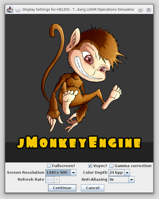
Figure 3: Choosing windows size and resolution at HELIOS start

After clicking ‘Continue’, the HELIOS graphical user interface (GUI) should appear (Figure 4):

Figure 4: HELIOS GUI with the control element bar left and the virtual scene and scanning animation filling the rest of the window

Navigation

You can turn the scene by clicking and holding the left or right mouse key and dragging the mouse in any direction. The scanning device will always be in the center of the window. Turning the mouse wheel will zoom in or out.

For more ways of navigating through a scene see the comprehensive manual.

Control element bar

Hint: If not all buttons are represented as in Figure 4, you have to change the screen resolution in the respective screen at startup (Figure 3).

Figure 5: Control element bar

1. Save Survey XML: Save survey to XML-file with survey information
2. Enable Free Camera: Change camera control from chase mode to free mode
3. Clear Points Buffer: Deletes already scanned (yellow) areas
4. Exit: Exit simulation, close window
5. Play: Start Scanning Simulation
6. Slower: Slow down the speed of scanning
7. Faster: Fasten the speed of scanning
8. Back: Go back to last waypoint
9. Next: Go to next waypoint
10. Add New: Add new waypoint at favored place with arrow keys
11. Delete: Delete one waypoint
12. Move: Move one waypoint to another place with arrow keys
13. Auto-Ground: adjust the scan position to the ground level
14. Edit Scan Field: Edit the extent of the scanners view
15. Scanner Active: Activate or deactivate scanning process
16. Head Rot (deg/sec): change the scanner’s head rotation with double click
17. Pulse Freq. (Hz): change the scanner’s pulse frequency with double click
18. Scan Freq. (Hz): change the scanning frequency with double click
19. Scan Angle: change the scanning angle with double click
20. Apply: operate given settings

Adding/moving scan positions

To add a new scan position, click the “Add New”-button in the control element bar. You can move the new scan position with the arrow keys your favored position.

To move an existing scan position, click the “Move”-button in the control element bar. Again, you can move the scan position with the arrow keys to a new position.

You can use the “Auto-Ground”-button to automatically adjust the scan position to the ground level. To move the scan position above the ground, deactivate the “Auto-Ground”-button.

Changing the scan field extent

The blue circle around the scanning devices in Figure 4 shows the horizontal extent of the scan. To adjust the scanned sector, click on ‘Edit Scan Field’ and increase/decrease the sector size with the up/down button of the keyboard (Figure 6). To turn the sector, use the right/left buttons.

Figure 6: Adjusted horizontal scan sector extent and orientation

Running the scan simulation

When satisfied with the scan sector, the scan simulation can be run with ‘Play’.

The simulated point cloud is visualized with yellow points.

The resulting point cloud is stored in
/HELIOS/output/Survey Playback/[name of survey as defined in survey .xml]/[time stamp of simulation start]/points/[number of scan position].xyz,
e.g. /HELIOS/output/Survey Playback/TLS Arbaro/2016-09-28_15-17-52/points/leg000_points.xyz

Output point cloud

The simulated point cloud consists of XYZ coordinates and full-waveform attributes in the following format (following the LAS 1.4 standard):

XYZ Intensity ECHO_WIDTH RN NOR FWF_ID OBJ_ID CLASS

see FWF.md for details. OBJ_ID is the ID of the respective object in the scene starting with ‘0’ and corresponding to the order of objects as stored in the scene .xml file.

Example output:
-16.480 -9.611 0.001 9808.5111 1.1461 1 1 24440 0 0
-16.637 -9.611 0.002 9787.4688 1.1461 1 1 24439 0 0
-16.793 -9.612 0.001 9766.2739 1.1462 1 1 24438 0 0
-16.949 -9.612 0.003 9744.9274 1.1462 1 1 24437 0 0
-17.261 -9.613 0.007 9701.7837 1.1463 1 1 24435 0 0
-17.420 -9.614 -0.001 9679.9885 1.1463 1 1 24434 0 0
-22.051 -9.631 -0.008 8988.1607 1.1471 1 1 24405 0 0
-16.169 -9.609 0.001 9850.1339 1.1461 1 1 24442 0 0