On Simulating Energy Consumption of Federated Learning Systems

This repository aim to provide a simulation of energy consumption of a federated learning system based on the non-orthogonal multiple access (NOMA) transmission protocols, proposed by Mo et. al. Energy consumption is computed during training along with energy consumed by communications between local machines and the server.

How to run software

1. Extract file .gz in folder "dataset" to binary file
2. Access to main.m and Run software in the MATLAB software
3. Install additional toolboxes (Deep Learning Toolbox and Communications Toolbox) ⓘ
4. Click "Run" button in under "Editor" tab in menu bar
5. Adjust a number of local iteration (ℕ) and global iteration (𝕄) on line 3 and 4 in "main.m" to simulate energy consumption. The output will show in "Command window" or in graph.
    

Project Description

A simulation of energy consumption of a federated learning system consists of one central server and a set of 𝒦 ≜ {1,2, ...,n-1, n} local machines (in Figure, each hospital are shown as a local machine)       
credit : https://rb.gy/bc4zmm

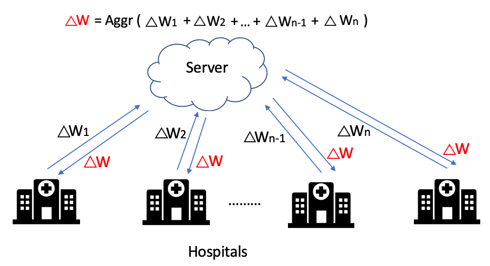
In general, the federated learning system would follow the 4 steps below.

1. central server broadcast global weight to local machines: The server broadcasts the global weight (Δ𝑤) to each local machines
2. local machine updates local weights each local machine updates its local weight in a local iteration (ℕ) to minimize the loss function.
3. local machines upload local weights to the central server The local machines upload their updated local weight Δ𝑤₁, Δ𝑤₂, . . , Δ𝑤_n-1, Δ𝑤_n to the server.
4. central server aggregate local weight and updated global weights The server aggregates all the uploaded local weight from n local machines and updates the global weight (Δ𝑤) by averaging them

From step 1 to 4, the process would repeat in a global iteration (𝕄)

This project set up has 1 central server and 3 local machines. The configuration in a central server and each local machines are in folder "class"

Software Structure

The structure of this project is as shown below the table.

	Description
class/...
- cnn_model.m	cnn_model() : this project uses CNN to minimize the loss function. If you want to use another algorithm, you can ignore this file.
- communication.m	communication() : This file use to config signal transmission parameters i.e. noise power at the server, the distance between each local machine and server, etc. in NOMA transmission protocol.
- device.m	device() : Configuration in each local machine parameter i.e. train and test dataset, transmission power, CPU cycle, achievable rate, etc.
- server.m	server() : Configuration in central server parameter i.e. train and test dataset, etc.
dataset/..	The train and test dataset would locate in this folder.
main.m	Use this file to run this project which would call the related function to follow these steps: 1. Train model at the server to provide an initial global weight to each local machine (call cnn_train()) 2. Each local machine receive a global weight(Δ𝑤) then call cnn_train() to minimize the loss function, then call time_at_loc() and energy_at_loc() to calculate time and energy consumption in computational part at each local machine3. The updated weight from each local machine after minimizing the loss function would be converted to a signal by call build_data_to_signal() 4. The signal from each local machine would be sent to the central server via NOMA protocol by call comm_to_server() 5. Central server would receive a signal which considers noise from communication (AWGN). Updated weights in the signal form are decoded to data by calling decode_at_server() and build_signal_to_data() 6. Time and energy consumption from communication would be calculated by calling time_and_energy_upload() 7. Central server would use aggregate_weight() to aggregate the updated weight from each local machine and calculate new global weight. the 1 to 7 step would be repeat in a global iteration (𝕄)

1.cnn_train()

To minimize loss function by using CNN, we call cnn_train() which implement in Lenet-1 structure. This function would return updated local weight and model accuracy.

[w1, w2, accuracy] = cnn_train(x_train, y_train, x_test, y_test, w1, w2, N)

Input	Description
x_train	train data sample
y_train	labeled data of train data sample
x_test	test data sample
y_test	labeled data of test data sample
w1	initial weight for 1st convolution layer in Lenet-1 architecture
w2	initial weight for 2nd convolution layer in Lenet-1 architecture
N	number of local iteration to train model (ℕ)
Output	Description
w1	updated weight for 1st convolution layer in Lenet-1
w2	updated weight for 2nd convolution layer in Lenet-1
accuracy	accuracy of the model after minimizing loss function

flop() If you did not use CNN to minimize loss function, you can use this function flop() to calculate a number of flop instead of the number of flop in cnn_model class (cnn_model.flop())

flop = flop(a, dataset)

Input	Description
a	number of FLOPs/each data sample per local update
dataset	data sample that use to minimize a loss function (Dk)
Output	Description
flop	the total number of FLOPs required at local machine (Fk)

2. time_at_loc()

You can use time_at_loc() to calculate the computation time at each local machine that uses in model training.

loc_time = time_at_loc(device,N)

Input	Description
device	local machine object that you want to find the computation time
N	number of local iteration to train model (ℕ)
Output	Description
loc_time	the computation time at local machine

3. energy_at_loc()

Energy consumption at the local machines are estimated by using energy_at_loc()

loc_energy = energy_at_loc(device, N)

Input	Description
device	local machine object that you want to find the energy consumption
N	number of local iteration to train model (ℕ)
Output	Description
loc_energy	energy consumption at local machine

4. build_data_to_signal()

The updated weight from model training must be prepared before transmission to a central server. So, we have to build a signal from updated weight by converted to binary form (in 32 bits, IEEE754-Single precision floating-point number format)

signal = build_data_to_signal(data)

Input	Description
data	updated weight from each local machine in string format
Output	Description
signal	updated weight in binary data format

5. comm_to_server()

When prepared binary data to build a signal to transmit to a central server, you will use comm_to_server() to simulate the actual communication network via NOMA transmission protocol which considered data modulation, the distance between local machines and server, superposition encoding, and signal combining.

[device1,device2,device3] = comm_to_server(device1,device2,device3,server, time_limit)

Input	Description
device1	local machine object #1 that you want to transmit signal
device2	local machine object #2 that you want to transmit signal
device3	local machine object #3 that you want to transmit signal
server	central server object
time_limit	the maximum duration time limit in second that you allow sending a signal for each time
Output	Description
device1	local machine object #1 that you want to transmit signal
device2	local machine object #2 that you want to transmit signal
device3	local machine object #3 that you want to transmit signal

6. decode_at_server()

On the central server side, the received signal that are sent via NOMA protocol would include additive white Gaussian noise (AWGN) which come from communication process. The received signal would be decoded by demodulation to get a signal from each local machine.

[device1,device2,device3] = decode_at_server(device1,device2,device3,rx_signal, time_limit)

Input	Description
device1	local machine object #1 that you want to transmit signal
device2	local machine object #2 that you want to transmit signal
device3	local machine object #3 that you want to transmit signal
rx_signal	received signal at central server from all local machine
time_limit	the maximum duration time limit in second that you allow sending a signal for each time
Output	Description
device1	local machine object #1 that you want to transmit signal
device2	local machine object #2 that you want to transmit signal
device3	local machine object #3 that you want to transmit signal

6. build_signal_to_data()

The decoded signal at the server is in decimal format. We have to convert the data format that we have to convert and shape data in a format that can use to do a weight aggregation process and use as an initial weight for the next global iteration (𝕄).

[bin_to_data_marray_w1, bin_to_data_marray_w2] = build_signal_to_data(signal_decode)

Input	Description
signal_decode	decoded signal from each local machine
Output	Description
bin_to_data_marray_w1	weight from the signal that readies for weight aggregation process at a central server (for convolution layer 1 in CNN which based on Lenet-1 architecture)
bin_to_data_marray_w2	weight from the signal that readies for weight aggregation process at a central server (for convolution layer 2 in CNN which based on Lenet-1 architecture)

7. time_and_energy_upload()

The duration time since a transmit signal from each local machine until the central server receives the whole part of the signal would be used to estimate energy consumption in the communication part. So, time_and_energy_upload would consider these conditions to calculate.

device = time_and_energy_upload(device, time_limit)

Input	Description
device	array of local machine object that you want to find the energy consumption
time_limit	the maximum duration time limit in second that you allow sending a signal for each time
Output	Description
device	array of local machine object

8. aggregate_weight()

The aggregate_weight() function would aggregate and find an average of updated weight that the server received and decoded from each local machine to update a new global weight. Then, the central server would provide a new updated global weight to the local machine to be an initial weight in each global iteration.

[w1, w2] = aggregate_weight(device)

Input	Description
device	array of local machine object
Output	Description
w1	updated global weight (Δ𝑤) for 1st convolution layer in Lenet-1
w2	updated global weight (Δ𝑤) for 2nd convolution layer in Lenet-1

9. total_time_noma()

The summation of time from computational and communication part via NOMA protocol in this federated learning system that we set it up by considering a global iteration(𝕄) and local iteration(ℕ) .

time = total_time_noma(t_local, t_upload, M, N)

Input	Description
t_local	computational time in model training (which is minimizing loss function)
t_upload	communication time in uploading an updated weight from each local machine to central server
M	the number of global iteration
N	the number of local iteration
Output	Description
time	total from computational and communication part via NOMA in this setting

10. display_output()

To visualization and show the experiment result as a graph or output in command line, we use display_output() to display our result.

display_output(device,keep,M,N,k,type)

Input	Description
device	array of local machine object
keep	the trigger to check that you want to keep a history of old data from previous experiment or not. If yes keep would be not empty, and no when keep is empty value
M	the number of global iteration
N	the number of local iteration
k	the number of local machine
type	type id of visualization result

Datasets

Our considered datasets, MNIST are located in folder “dataset”. If you want to use another dataset you can place it in this path and then change a file configuration in the file “class/device.m” (line 42-46) and “class/server.m” (line 18-21)

Experiment Setting

• 1 central server and 3 local machines.
• Setting at Central server : (MNIST train/test dataset - 8,000/2,000 samples)
  • test dataset : MNIST 2,000 samples
• Setting at Local machine
  • local machine#1 : (MNIST train/test dataset - 300/1,000 samples), CPU model = Cortex-A76
  • local machine#2 : (MNIST train/test dataset - 300/1,000 samples), CPU model = Samsung-M1
  • local machine#3 : (MNIST train/test dataset - 400/1,000 samples), CPU model = Cortex-A76

parameter	machine#1	machine#2	machine#3	Description
si	0.0045x10-21	0.0049x10-21	0.0045x10-21	Const. coefficient depend on chip architecture
p_tx_db	21	27	21	Transmission power in dB @ local machine
f	3x109 (Hz)	2.6x109 (Hz)	3x109 (Hz)	CPU frequencY_train of whole operation duration
c	16 (Flop/Cycle)	6 (Flop/Cycle)	16 (Flop/Cycle)	the number of FLOPs in CPU cycle
d	100 (m)	150 (m)	200 (m)	distance between Device to Server

• Setting in CNN Model : Lenet-1 architecture LeNet-1 was initially trained on LeCun’s USPS database, where it incurred a 1.7% error rate. LeNet-1 was a small CNN, which merely included five layers. The network was developed to accommodate minute, single-channel images of size (28×28). It boasted a total of 3,246 trainable parameters and 139,402 connections. This processing was done by using a customised input layer. The five layers of the LeNet-1 were as follows:
  • imageInputLayer: input size = [28x28]
  • Layer C1: Convolution Layer (num_kernels=4, kernel_size=5×5, padding=0, stride=1) - [5x5x4]
  • Layer S2: Average Pooling Layer (kernel_size=2×2, padding=0, stride=2) - [2x2]
  • Layer C3: Convolution Layer (num_kernels=12, kernel_size=5×5, padding=0, stride=1) - [5x5x12]
  • Layer S4: Average Pooling Layer (kernel_size=2×2, padding=0, stride=2) - [2x2]
  • Layer F5: Fully Connected Layer (out_features=10) - [10]
• Setting in communication part

parameter	value	description
path_loss_exp	3	path loss exponent
d_0	1 (m)	reference distance
d_1	100 (m)	distance between machine#1 to central server
d_2	150 (m)	distance between machine#2 to central server
d_3	200 (m)	distance between machine#3 to central server
d_max	500 (m)	maximum distance for attenuation calculation
h_0	30	channel power gain at a reference distance of d_0 --> β_0
bw	2x106 (Hz)	bandwidth
noise_power_db	-100 (dBm/Hz)	noise power @ server (in dBm)

Reference

• Energy-Efficient Federated Edge Learning with Joint Communication and Computation Design by Mo et. al.
• Y. LeCun, B. Boser, J.S. Denker, D. Henderson, R.E. Howard, W. Hubbard, and L.D. Jackel, Handwritten digit recognition with a back-propagation network (1990), In Touretzky, D., editor, Advances in Neural Information Processing Systems 2 (NIPS*89), Denver, CO. Morgan Kaufmann