Link to calculator: https://rohanphanse.github.io/calculator
An intuitive and easy-to-use web calculator with the power of functional programming languages and the terminal!
My goal for this project was to create a web calculator that offered standard calculator functions as well as more powerful features from programming languages through a simple and accessible syntax.
As a challenge to myself, I decided not to use any external libraries. The entire calculator including the parser, evaluation engine, and UI was implemented with a few thousand lines of JavaScript code!
Math Features: linear algebra (e.g. rref and eigen), calculus (e.g. diff and lim), complex numbers, polynomial root solvers, 2D graphing with plot, 3D graphing with plot3
Physics and Chemistry Features: physical units and constants, molar masses, balance chemical equations
Functional Programming Features: variables, regular and anonymous @ functions, map and filter, type checking, lambda capture, currying, conditional logic, trace function calls
Terminal Features: arrow keys move through history, help documentation, syntax highlighting, autocomplete
Additional Features: locally save variables and functions, unit and base conversions
Here is a brief tutorial on Functional Calculator's language in the style of Learn X in Y minutes:
----------------------------------------------------
-- 1. Numbers
----------------------------------------------------
-- All the following are treated as type `number`:
3 -- 3 (integer)
3.14 -- 3.14 (floating point)
3.14e+5 -- 314000 (scientific notation)
0b101 -- 0b101 (5 in binary)
0xdecaf -- 0xdecaf (912559 in hexadecimal)
0o12 -- 0o12 (10 in octal)
20/6 -- 10/3 (fraction)
5 km -- 5 km (number with unit)
4 + 2i -- 4 + 2i (complex number)
-- Tip: use `type(x)` to check the type of `x`
type(4 + 2i) -- number
-- Tip: use `help func` to learn about `func`
help +
-- Name: Addition
-- Usage: a + b
-- Types: a: number | list[any], b: number | list[any]
-- Examples:
-- 1. Add numbers: 2 + 2 -> 4
-- 2. Add tensors: [[[1, 2]]] + [[[2, 1]]] -> [[[3, 3]]]
-- 3. Add numbers and tensors: 2 + [1, 2] -> [3, 4]
-- Operators are overloaded to work with various kinds of numbers:
-- For example, the exponentiation operator behaves in multiple ways:
3^2 -- 9
(5 km)^2 -- 25 km^2
(4 + 2i)^3 -- 16 + 88i
-- Math operators: +, -, * , /, ^, !, mod
-- Bitwise operators: <<, >>, ~, &, |, xor
-- Base conversions: bin, hex, oct, dec
0b110 xor 1 -- 7
bin 7 -- 0b111
----------------------------------------------------
-- 2. Variables and Functions
----------------------------------------------------
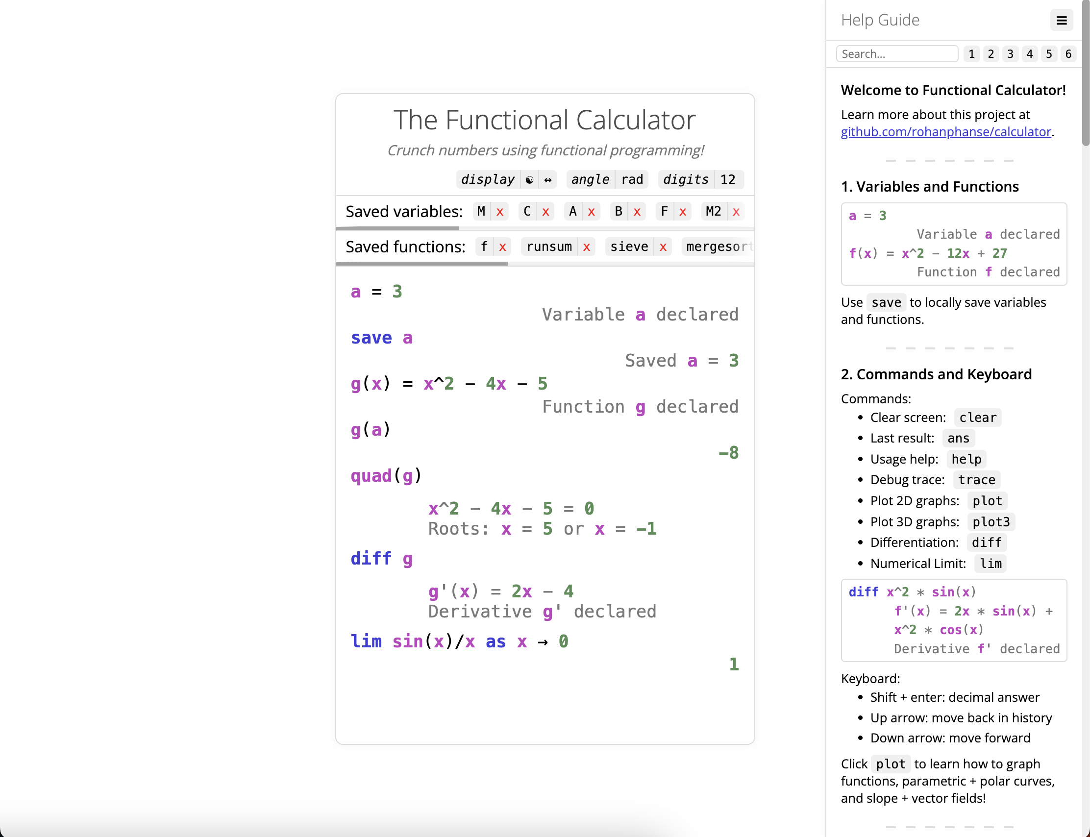
a = 3 -- Variable a declared
2a + 1 -- 7
f(x) = x^2 - 12x + 27 -- Function f declared
f(0) -- 27
add(a, b) = a + b -- Function add declared
-- Tip: locally save variables and functions with `save`
save a -- Saved a = 3
save f -- Saved f(x) = x^2 - 12x + 27
-- We can also define `add` using a lambda function
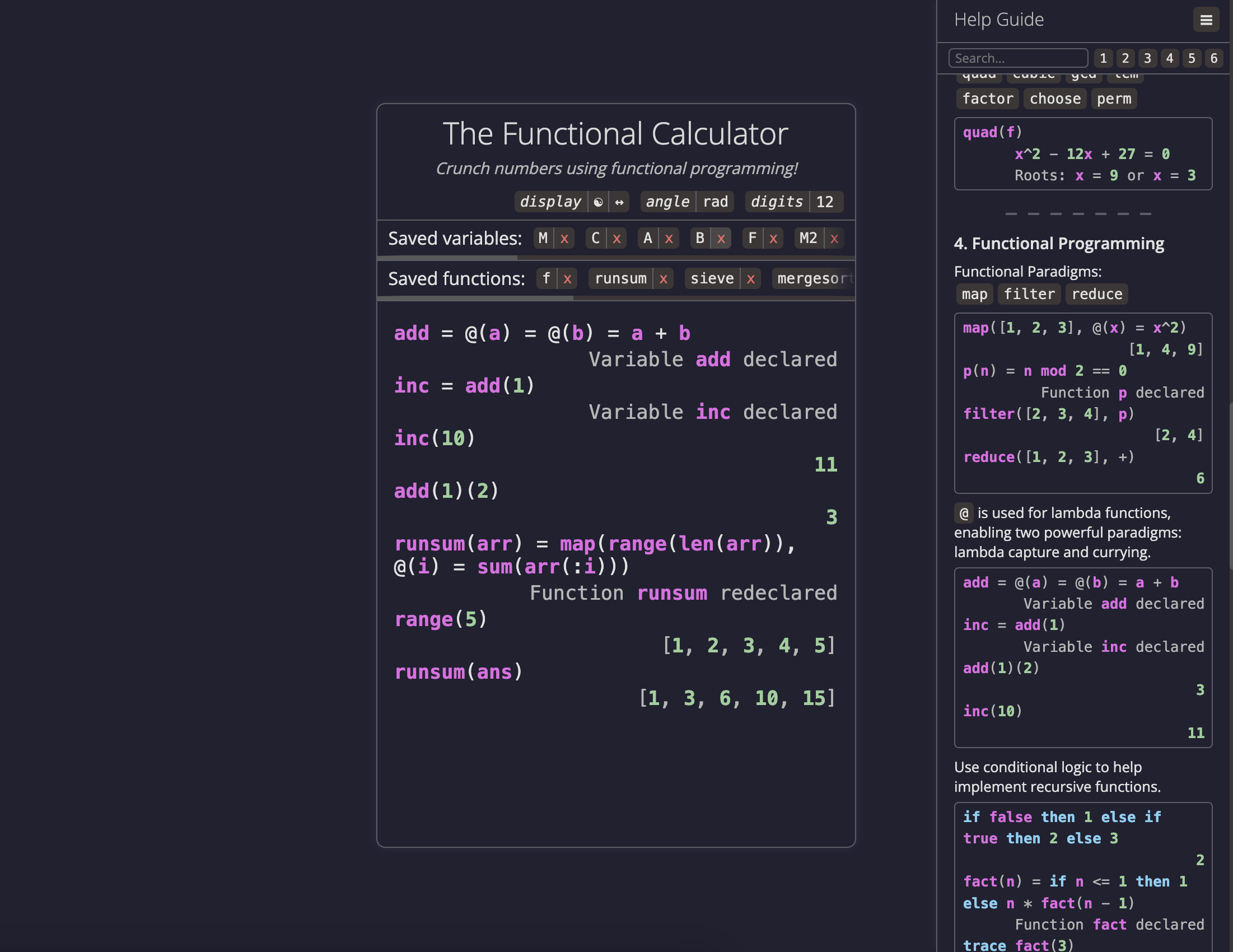
add2 = @(a, b) = a + b -- Function add2 declared
add2(1, 2) -- 3
-- In fact, let's try nested lambda functions
add3 = @(a) = @(b) = a + b -- Function add3 declared
add3(1)(2) -- 3
-- Thanks to lambda capture, we can partially apply `add3`
-- to create an incrementer function `inc`
inc = add3(1) -- Function inc declared
inc(10) -- 11
----------------------------------------------------
-- 3. Lists
----------------------------------------------------
type [1, 2, 3] -- list[number]
type [[1, 2], [3, 4]] -- list[list[number]]
type [1, [2]] -- list[any]
-- List indexing (one-based):
M = [[1, 2], [3, 4]] -- Variable M declared
M(2) -- [3, 4]
M(2, 1) -- 3
M(:, 1) -- [1, 3] (first column of `M`)
X = [2, 3, 5, 7] -- Variable X declared
X(:2) -- [2, 3]
X(2:) -- [3, 5, 7]
X(2:3) -- [3, 5]
-- List utilities: range, len, concat
range(3) -- [1, 2, 3]
range(3, 5) -- [3, 4, 5]
len([0, 0]) -- 2
concat([1, 2], [3, 4]) -- [1, 2, 3, 4]
concat([1, 2], 3, 4) -- [1, 2, 3, 4]
----------------------------------------------------
-- 4. Conditional Logic
----------------------------------------------------
-- Booleans (type: `bool`):
true -- true
false -- false
-- Boolean operators: ==, !=, <, >, <=, >=, and, or, not
5 mod 2 == 1 -- true
3 < 4 and not true -- false
-- Conditional Statements
if false then 1 else 2 -- 2
sign(x) = if x > 0 then 1 else if x < 0
then -1 else 0 -- Function sign declared
sign(-10) -- -1
----------------------------------------------------
-- 5. Functional Programming
----------------------------------------------------
-- Here are some helpful functions from functional programming:
-- 1. `map(X: list[any], f: function)` - apply `f` to each element of `X`
-- 2. `filter(X: list[any], f: function)` -- keeps elements of `X` where
-- `f` returns true
-- 3. `reduce(X: list[any], f: function)` -- combines elements of `X` into
-- one value using `f`, from left to right
map([1, 2, 3], @(x) = x^2) -- [1, 4, 9]
p(n) = n mod 2 == 0 -- Function p declared
filter([2, 3, 4], p) -- [2, 4]
reduce([1, 2, 3], +) -- 6
-- Tip: use `trace` to help with debugging recursive functions
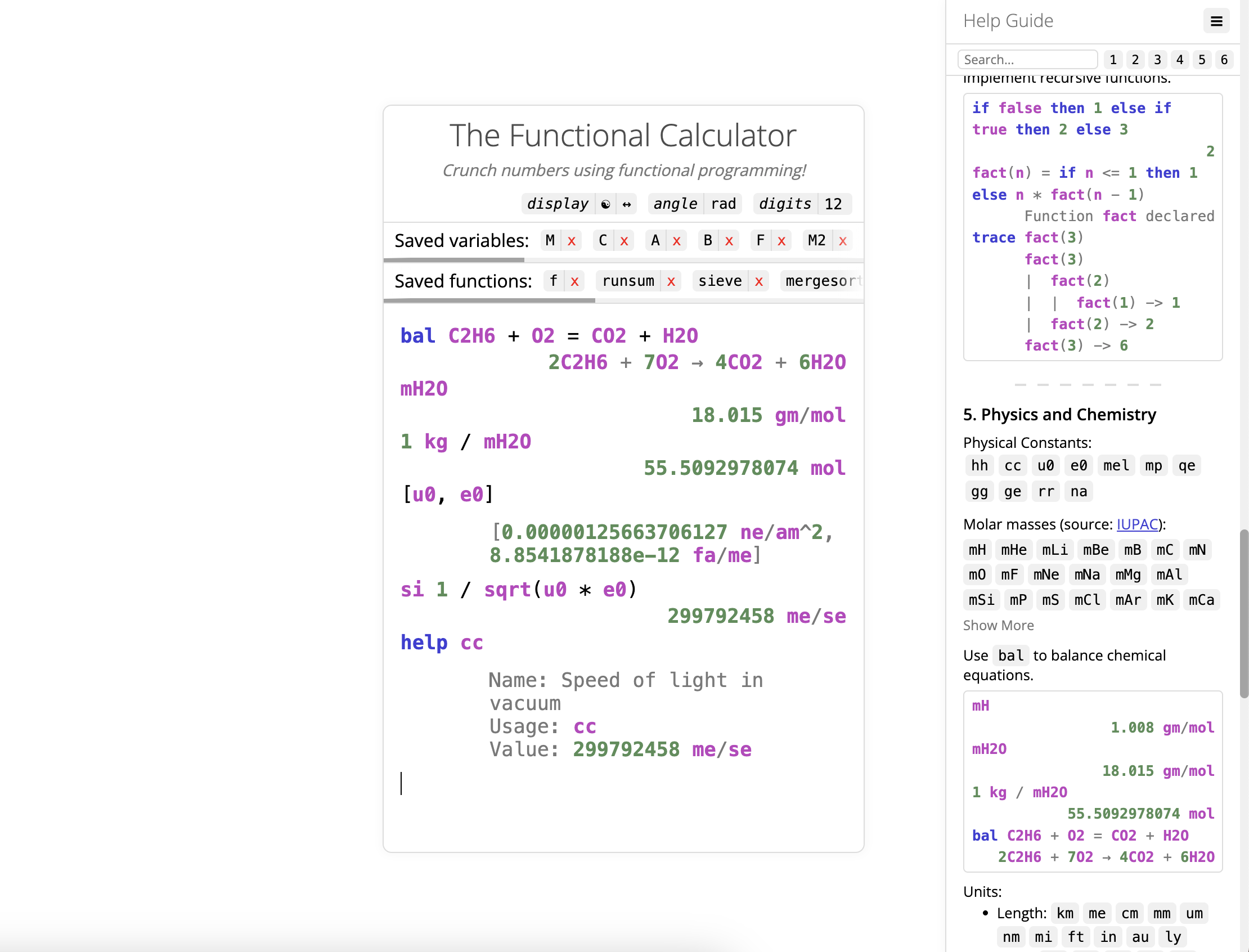
fact(n) = if n <= 1 then 1 else n * fact(n - 1) -- Function fact declared
trace fact(3)
-- fact(3)
-- | fact(2)
-- | | fact(1) -> 1
-- | fact(2) -> 2
-- fact(3) -> 6
----------------------------------------------------
-- 6. Math
----------------------------------------------------
-- Math functions: log, ln, sqrt, abs, ceil, floor, round
-- Trigonometry: sin, cos, tan, arcsin, arccos, arctan, csc, sec, cot
-- Math constants: pi, e, phi, i
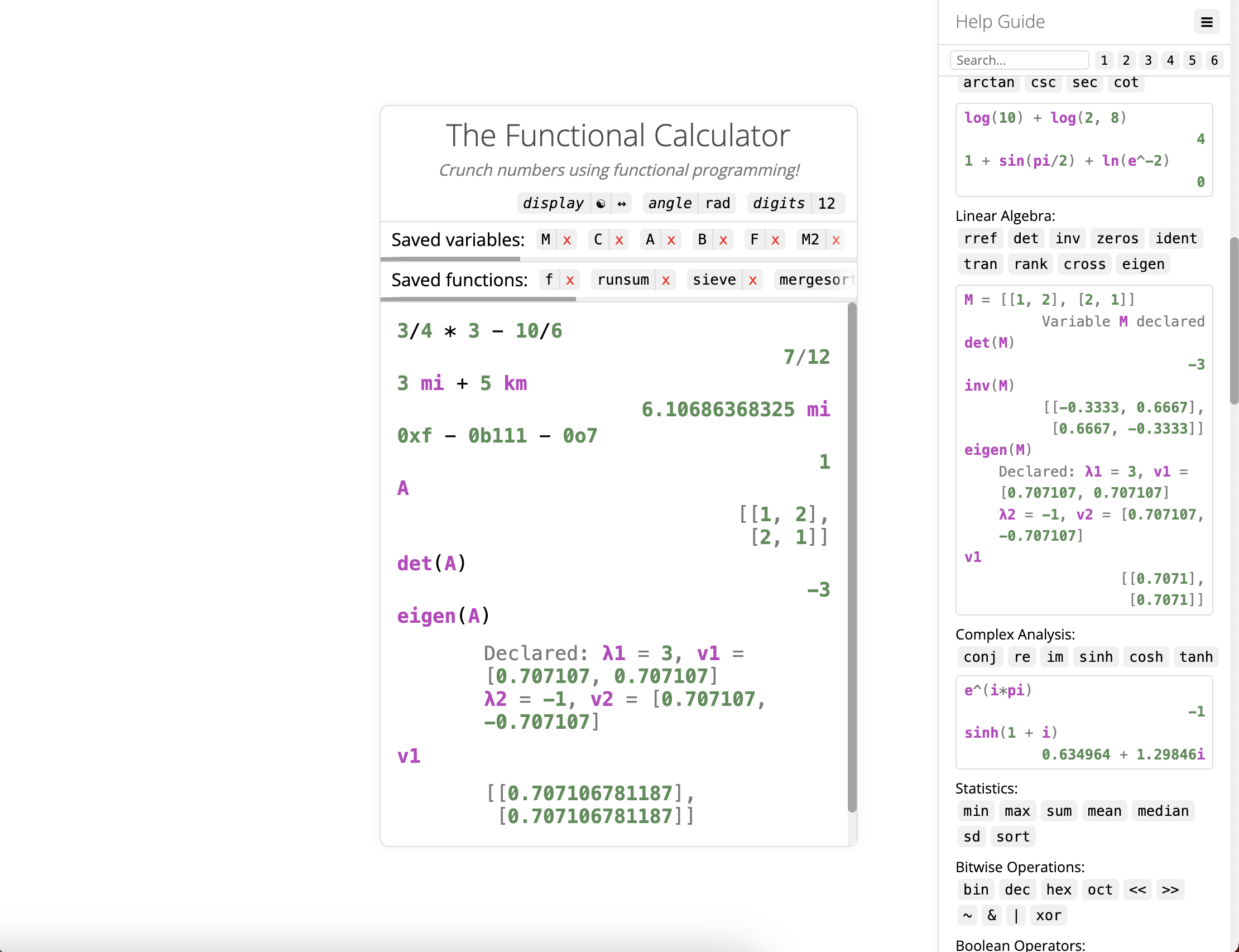
log(10) + log(2, 8) -- 4
1 + sin(pi/2) + ln(e^-2) -- 0
-- Linear algebra: rref, det, inv, zeros, ident, tran, rank, cross, eigen
M = [[1, 2], [2, 1]] -- Variable M declared
det(M) -- -3
inv(M)
-- [[-0.3333, 0.6667],
-- [0.6667, -0.3333]]
eigen(M)
-- Declared: λ1 = 3, v1 = [0.707107, 0.707107]
-- λ2 = -1, v2 = [0.707107, -0.707107]
v1
-- [[0.7071],
-- [0.7071]]
-- Calculus:
-- 1. Perform symbolic differentation with `diff`
-- 2. Compute numerical limits with `lim`
-- Tip: type the arrow in `lim` with the `\to` macro
diff x^2 * sin(x)
-- f'(x) = 2x * sin(x) + x^2 * cos(x)
-- Derivative f' declared
lim sin(y)/y as y → 0 -- 1
-- Complex analysis: conj, re, im, sinh, cosh, tanh
e^(i*pi) -- -1
sinh(1 + i) -- 0.634964 + 1.29846i
-- Statistics: min, max, sum, mean, median, sd, sort
-- Miscellaneous: quad, cubic, gcd, lcm, factor, choose, perm
----------------------------------------------------
-- 7. Physics and Chemistry
----------------------------------------------------
-- Chemistry:
-- 1. The molar mass of molecule "X" is available as "mX"
-- 2. Use `bal` to balance chemical equations
mH -- 1.008 gm/mol
mH2O -- 18.015 gm/mol
1 kg / mH2O -- 55.5092978074 mol
bal C2H6 + O2 = CO2 + H2O -- 2C2H6 + 7O2 → 4CO2 + 6H2O
-- Physics:
-- 1. Use `to` to convert from one unit to another
-- 2. Use `si` to convert to SI units
5 km + 500 me -- 5.5 km
5 me / 2 se -- 2.5 me/se
u0 -- 0.00000125663706127 ne/am^2
e0 -- 8.8541878188e-12 fa/me
si 1 / sqrt(u0 * e0) -- 299792458 me/se
cc to km to ms -- 299.792458 km/ms
help cc
-- Name: Speed of light in vacuum
-- Usage: cc
-- Value: 299792458 me/se
----------------------------------------------------
-- 7. 2D and 3D Graphing
----------------------------------------------------
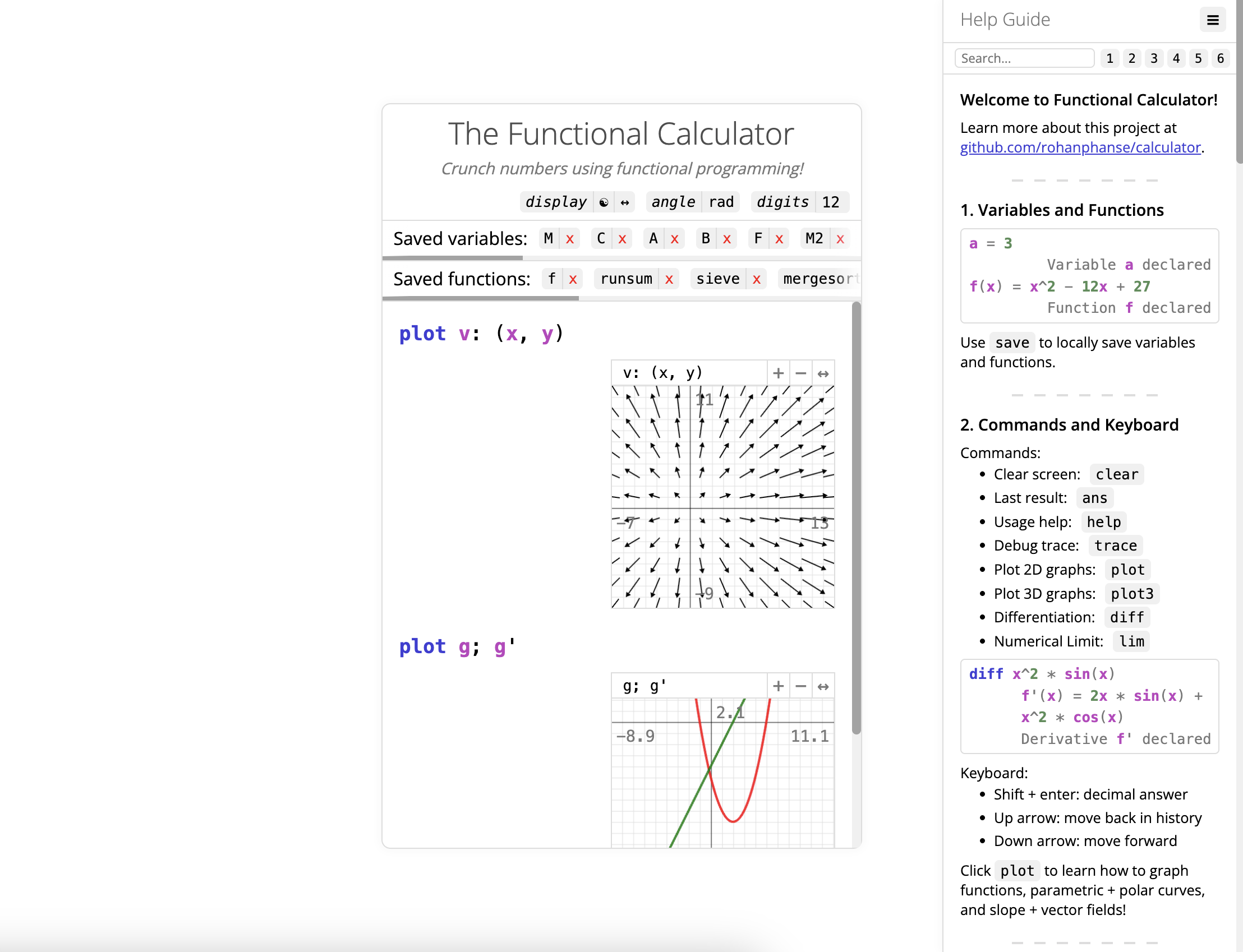
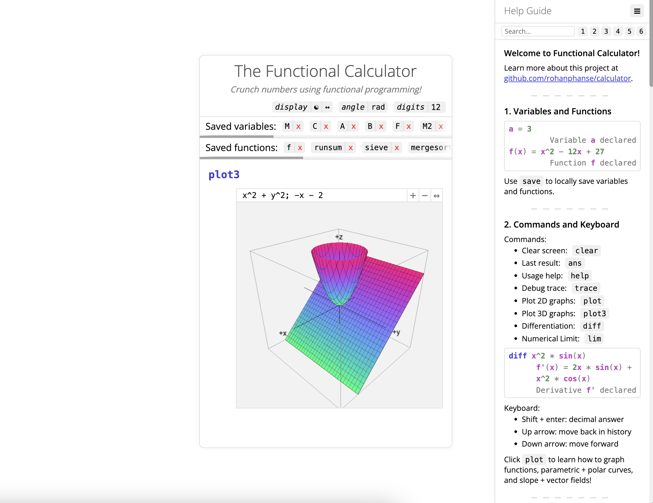
-- Use `plot` to graph in 2D and `plot3` for 3D
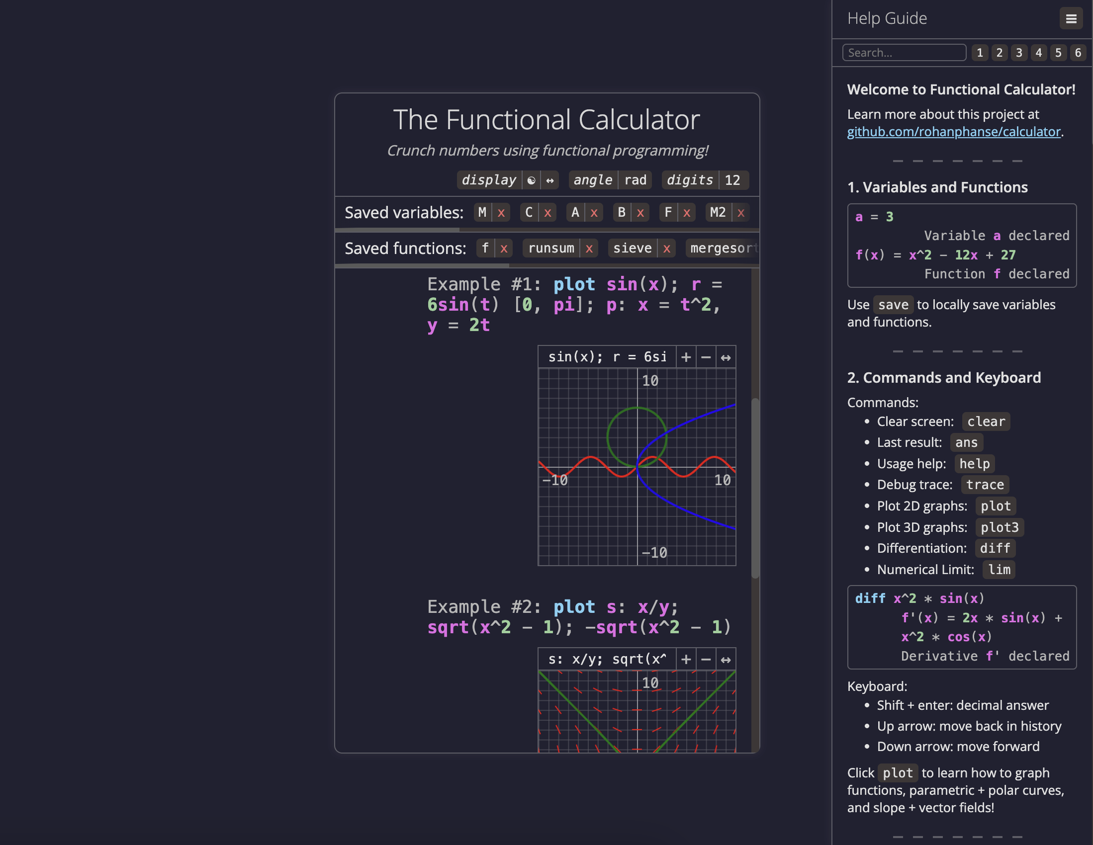
-- Guide to `plot`:
-- 1. Graph functions of x as f(x)
-- 2. Polar curves: r = f(t)
-- 3. Parametric: p: x = f(t), y = g(t)
-- 4. Slope fields: s: f(x, y)
-- 5. Vector fields: v: (f(x, y), g(x, y))
plot sin(x); r = 6sin(t) [0, pi]; p: x = t^2, y = 2t
plot s: x/y; sqrt(x^2 - 1); -sqrt(x^2 - 1)
plot v: (x, y)
-- Guide to `plot3`:
-- 1. Graph functions of x and y as f(x, y)
plot3 y^2 - x^2