Time based simulation
In order to simulate the constant data stream from the detector, time based simulation concept has been introduced to FairRoot. This step is usually performed during digitisation of data from individual detectors. It is the responsibility of various detector groups to properly introduce the detector response. Running of the time based simulation is triggered via functions in FairRunAna. One may simulate events’ start times according to Poissonian distribution (with a mean time between events as the parameter) or with a constant probability between given minimum and maximum times:
fRunAna->SetEventMeanTime(Double_t mean);
fRunAna->SetEventTimeInterval(Double_t min, Double_t max);
The standard way of running analysis is quite strictly event-based. Data from each event are processed separately and independently from data in other events. The simulation of a continuous data stream requires combining data from different events. It is achieved with the help of individual data handlers that derive from FairWriteoutBuffer.
The standard way of storing data by tasks are to register the output TClonesArrays in the FairRootManager and then to store data in the output TClonesArray for each event. Some of these TClonesArrays (“persistent” ones) are saved after each event to the output tree by FairRunAna.
The tasks designed to run in the time based mode are creating instance of the MyDataWriteoutBuffer in the initialisation stage. The data are added to the MyDataWriteoutBuffer with the StartTime and EndTime.
fMyDataWriteoutBuffer->FillNewData(MyData,StartTime,EndTime);The StartTime and EndTime indicate the time, when the MyData can be influenced by or can influence the later coming data. If such thing happen, i.e. if there will come a new data with StartTime laying between MyData’s StartTime and EndTime, then MyDataWriteoutBuffer::Modify() function will be called. This, very detector-specific function, defines the way the two conflicting data are modified.
Remark: usually any detector has many channels that are working independently. The operator MyData::operator==() is used to check if the data can influence each other.
After each event MyDataWriteoutBuffer is checking the data in the buffer selecting the ones that have EndTime smaller than this EventStartTime. These data that have no chance of being modified any more, will be stored on the disk.
After all events are processed, the rest of the created data are stored in one extra event at the end of the tree.
It is advisable to write a MyDataSorterTask that will sort the objects of MyData in the output array to facilitate the access to the data in the reconstruction stage.
The standard way of getting data inside the task it to request the pointer to the TClonesArray from the FairRootManager instance.
inputArray = (TClonesArray*) rootManager->GetObject(“MyInputData”);When accessing the data obtained in the time based mode one shouldn’t access the data from different events, as the data distribution is chopped by the simulated event structure. The data have to be accessed in realistic time chunks. In FairRoot such data access is enabled using binary functors. Currently two functors are implemented: *StopTime - returns all the data smaller than the time parameter. It does not return data requested before. *TimeGap - returns all the data till a gap in the data time stream of a given length.
BinaryFunctor* fFunctor  = new TimeGap(); // or StopTime();
Double_t       parameter = 20.;           // in nanoseconds
inputArray = (TClonesArray*) rootManager->GetData(“MyInputData”,fFunctor,parameter);
In the figure the data yield from an example detector is shown as a function of StartTime. The ActiveTime = StopTime-StartTime for this data type is set to 100ns.
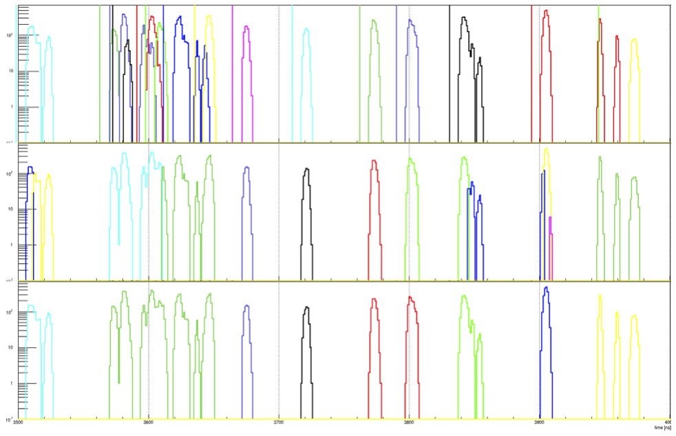
Event based digitization. The colour coding in the top panel is representing the simulated MonteCarlo event structure. The vertical lines represent the event start time, while the histogram of the same colour represents digitised data distribution from that event. The events are distributed randomly according to Poissonian distribution with mean time of 50ns. The data for this specific detector is coming about 15ns after the EventStartTime with a width of about 10ns. The detector has data almost in every event. For some events there are data coming even hundreds of nanoseconds after the event start time.
Time based digitization. The middle panel shows the data structure as read directly from the tree with the digitised data (that shouldn’t be done). Different colours represented data stored in different tree entries. The data is often chopped in the middle of the original event’s distribution. It should also be noted that the colour changes (the tree entries boundaries) coincide with the original (EventStartTime-100ns), where the 100ns comes from the detector’s data ActiveTime.
TimeGap(20ns). The bottom panel presents the data retrieved with the BinaryFunctor* fFunctor = new TimeGap(); set to 20ns. The data slices, that the analysis tasks will be working on, are presented in different colours. As requested, these data slices are defined by gaps in the data stream with a length of 20ns or longer. Comparing with the simulated event structure (top panel) one can see, that the time slices do not correspond directly to the original events: quite often they enclose data from several events (like the “green” time slice around t=3600ns composed of data from 7 simulated events) and sometimes the data from one event is distributed over several time slices (like the “red” event around t~3900ns distributed over 2 time slices).